Assessing Policy Effectiveness to Measure Inequality of Opportunity in Wellbeing and Education: Case of Tunisia 

 

Bassma Said Jellali

University Taibah, Saudi Arabia.	Abstract This paper aims to examine the effects and evolution of unequal opportunities on the distribution of wellbeing indicators covering the period 2005 to 2010. We used parametric and non-parametric approach for well-being and Dissimilarity-Index for education. Father's education, residence area, and connection to drinking water appear to be the most important background variables affecting well-being profile. Child’s sex appears to be the most important determinant of the accessibility to education. Policy makers must make appropriate policies to reduce intergenerational transmission of parental background and sex discrimination and to overcome traps of inequality for future generations. We found that the place of residence with a contribution rate of 22.25%. Thus, the influence of the place of residence on the distribution of accessibility to education can be explained by the fact that the inhabitants of rural areas remain disadvantaged compared to urban dwellers in terms of lack of basic infrastructure (the distances that separate households from public primary or secondary establishments).
Licensed: This work is licensed under a Creative Commons Attribution 4.0 License.
Keywords: Dissimilarity index Inequality of opportunity Consumption Tunisia Public policy. JEL Classification: D31; D63; J62.
Accepted: 21 October 2019 Published: 11 November 2019

Funding: This study received no specific financial support.

Competing Interests:  The author declares that there are no conflicts of interests regarding the publication of this paper.

Acknowledgement:The author is grateful to an anonymous referee and the editor for many helpful comments and suggestions. Any errors or omissions are, however, our own.

1. Introduction

The term inequality of opportunity lies in the political philosophy initiated by Rawls (1971) whose objective was the search for an ethically acceptable social order. To this end, the search for equality in well-being measured by the utility proposed by the welfarist tradition is strongly criticized because it does not hold individuals accountable for their responsibilities, preferences or choices. According to Roemer (1993), Peragine (2004), Ramos and Van De Gaer (2016) inequalities on the distributions of human development indicators can be explained by two types of factors: The factors that individuals are not responsible for or circumstances and the factors that individuals are held accountable for and that are part of their efforts. In contexts where the inequalities of opportunities are much accentuated, the social status of the parents for example conditions the level of the monetary incomes of the individuals. In general, the inequalities of opportunity that individuals face in a society need to be illuminated for three reasons: (i) Inequalities of opportunity constitute an unacceptable social injustice because ideally only the efforts of individuals explain inequalities (Kolm, 1996). (ii) Only economic policies designed to reduce inequalities of opportunity are of interest as the state should only compensate for inequalities of opportunity and allow individuals to compensate for the inequalities associated with their efforts (Arneson, 1989). (iii) According to the World Bank (2005), Ferreira and Gignoux (2008) countries where inequalities of opportunity are accentuated experience low economic growth rates because they discourage investments in human development. On the other hand, inequalities linked to personal efforts encourage investment in human capital, resulting in high rates of economic growth. It is understandable that controlled variables can become circumstances for future generations.

As for its scope of policy, it should be noted that since the work of Roemer (1993) the general tendency invites the public authorities to fight against the inequalities of opportunities rather than against the inequalities of the variables under control. In fact, when they want to fight against the inequalities linked to individual efforts, the public authorities generally apply two types of policies: the first is fiscal and consists in taxing citizens with progressive taxes in order to compensate for low wages. The second is based on quotas that allow groups disadvantaged by their poor performance to still be present in all public bodies and all training schools for the preparation of future leaders. According to Hassine (2011) such strategies that directly target the equality of well-being indicators result in the demotivation of individuals' efforts, the discouragement of investing in human resources and the annihilation of innovation.

According to this principle, inequalities of opportunity must be eliminated and we can measure them according to two approaches. The present study is part of the multidimensional approach of development as recommended by the United Nations Development Program (UNDP, 2014) and considers two indicators of human development as the monetary indicator and education.

The literature on the inequality of opportunities in the MENA region is limited but also in process; in particular because of data availability. For example, some studies show that there are high levels of inequality of opportunity in health and education access Assaad, Krafft, Hassine, and Salehi-Isfahani (2012).  Similarly, other works studied poverty and inequality in Tunisia (Ayadi, Boulila, Lahouel, & Montigny, 2005; World Bank, 1995). However, all research in the Tunisian context was limited to analyse the inequality of opportunity for access to basic services like electricity, drinking water, sanitation, education and health. To our knowledge, it does not have an attempt to study the extent of inequality of opportunity on the distribution of development in terms of monetary well-being and education access in this country.

In addition, traditional measures of inequality do not reflect precisely the reality and do not allow for fair and unjust inequalities to be taken into account.  For example, the level of inequality measured by the standard Gini index is not particularly high for the MENA countries (Bibi & Nabli, 2009; Hassine, 2015). A possible explanation for this "contradiction" is that the observed inequality may mask a significant portion of unjust and unjustifiable inequality associated with social class or other circumstances over which the individual has no control.

So we will study the effects of unequal opportunities on the distribution of monetary well-being indicators and education. For the robustness of our estimation, we apply firstly the parametric approach and the nonparametric approach to the monetary dimension captured by the final consumption of households. Then, we apply the dissimilarity indices on accessibility to basic education by children at school age. Our results show that, without efficient policies to reduce sex discrimination and intergenerational transmission of parental disadvantages, disparities in Tunisia may intensify.

The rest of the paper proceeds as follows: in section 2 we develop our conceptual framework discussing the different techniques to measure inequality of opportunity. In section 3 we describe our data set and explain main variables of interest. In section 4, we present our results and discussions. Section 5 concludes.

2. Conceptual Framework

All discussions on measures of inequality of opportunity must be guided by a number of principles (Ramos & Van De Gaer, 2016).The most important of which in the sense that it leads to concrete proposals for measurement are the principle of compensation. It requires that inequalities of opportunity must be neutral with respect to results. So, two approaches are proposed in the literature to distinguish ex-post and ex-ante inequality. Ex-ante equality is achieved when circumstances do not affect the results. However, ex-post inequality is excreted on effort, and it is reached when all individuals with the same effort achieve the same results.

2.1. Inequality of Opportunities: Distribution of Consumption

2.1.1. Measurement of the Inequality of Opportunities by the Parametric Approach

The measure of inequality requires the choice of an index of inequality. In our case we will use the generalized entropy index GE(0)¹ , it is the most recognized and the most used (Ferreira & Gignoux, 2011).

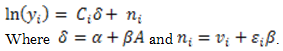
Whit    (because the circumstances also influence the efforts); α et β: are vectors of the coefficients, A is a matrix of coefficients that specify the effects of the circumstances on the forces and εi is an error term. Equation [2] can be written in a reduced form:

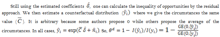
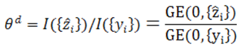
From the estimated coefficients   in [3], one can calculate a counterfactual distribution  where the inequality is only due to the circumstances. It is obtained simply by ignoring the error term  and . Essentially, predicted values ​​are used as estimates of means for types. Inequality between these means is a measure of inter-type inequality. If the linear relationship is maintained and there are no missing interaction terms, the results would be the same as for a nonparametric estimate. So the proportion of inequality of opportunity in total inequality is given by:

The direct and the indirect or residual methods may give different results. The only measure of inequality that gives the same results with both methods is the GE (0)² entropy measure. In addition to calculating the value of the inequality of opportunity, [3] also allows the decomposition by sources.  

2.1.2. Measure of Inequality of Opportunity by Non-Parametric Approach

2.1.2.1. The Direct Non-Parametric Approach

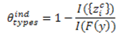
Following the approach by types, inequality of opportunity is measured by inequality between types. This inequality can be estimated directly by performing a smoothing that leads to consider constancy as a reference

2.1.2.2. The Indirect Nonparametric Approach

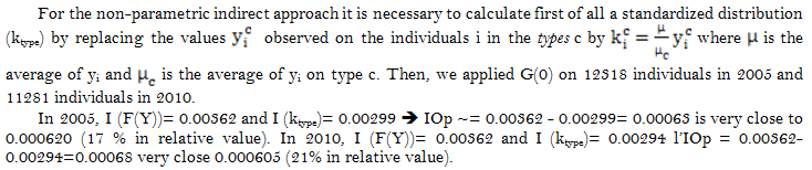
Inequality of opportunity can also be obtained indirectly through a standardized distribution obtained by replacing the values  observed on individuals i in types c by  where  is the overall average of yi and  is as previously defined, the average of yi on the type c (Ferreira & Gignoux, 2008). The standardized distribution eliminates all inter-type inequalities and leaves only intra-type or effort-related inequalities. We can then calculate inequality due to opportunities as following (Ramos & Van De Gaer, 2016):

If we want to express it in relative value, the proportion of the inequality of opportunities in the total inequality of yi is given by:

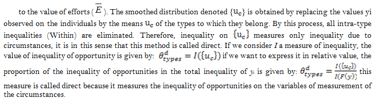
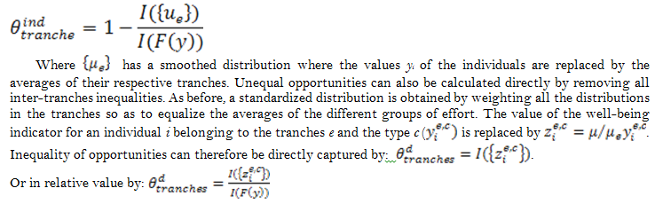
Following the approach by tranches, inequality of opportunity is measured by focusing on the distribution of yi within groups with the same efforts. As in the previous case, a smoothed distribution is calculated to eliminate all intra- tranches inequalities. Unequal opportunities are expressed by:

The share of inequality due to differences in opportunities is calculated by:

2.2. Inequality of Opportunity to Access Basic Education

2.2.1. Calculation of the Dissimilarity Index:  D-Index of Access to Basic Education

To study the differential distribution of a binary variable on a set of socio-economic variables, we chose the Dissimilarity-index noted D-index as a methodology developed by the World Bank (2009), Kovacevic (2010) and Yalonetzky (2012).

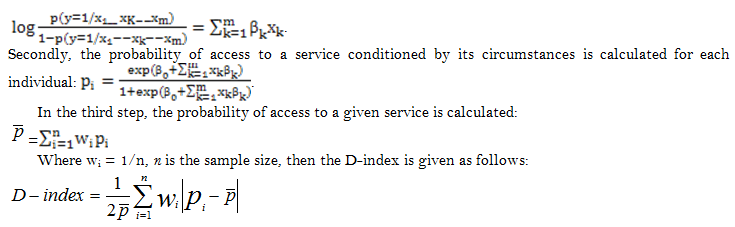
In practice, the D-index can be calculated in three steps:

Let x1,…,xk,…,xm be a set of circumstances associated with an individual i, then this individual is characterized by a vector of circumstances xi = x1i,…,xki,…,xmi.

Firstly, conditional probabilities can be evaluated by specifying a logistic function (or Probit) between accessibility to a dependent variable and circumstances by:

2.2.2. Shapley's Decomposition: Identifying which "Circumstances" Contribute to Inequality

To study the evolution of inequality and to measure the contributions of different variables of circumstances in inequality of opportunity, we use the decomposition procedure proposed by Shorrocks (2013) which is based on the Shapley value concept of cooperation games.

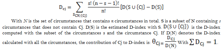
After defining the index of Dissimilarity (D-index), we can see that its value depends on the number of circumstances considered. Indeed, if the number of circumstances is high, D-index is large.

The marginal impact of a particular circumstance Cj is calculated by the value of Shapley (World Bank, 2012):

3. Data and Samples  

The 2005 and 2010 national surveys are carried by a random sample of 13,392 stratified households at 2 degrees. It should be noted that of the 13,392 sample households drawn, a total of 11,281 households were actually surveyed, which is 84.2% of the initial sample. These surveys provided information on socio-demographic characteristics such as household size, education level of the head of household, socio-professional category, such as the environment and the region of residence of the household. Despite these regular surveys and the ease of access to such data after the 2010 revolution, there is little research on inequality in Tunisia limited to the calculation of an index at the national level.

3.1. Monetary Dimension (Final Consumption): IOP of the Monetary Dimension

From these data, six hypothetical explanatory circumstances of the inequality on the monetary indicator were presented in the table below Table 1 the sex of the head of the household, inhabited areas, the living environment (rural or urban), the connection of households to the sewerage network, branching of households with drinking water, and connection of households to electricity. For the choice of our variables, we are based on important indicators and outcomes identified by previous works as contributing to explain inequality of opportunity access to basic services, and as constrained by the data availability (Jemmali & Amara, 2014; Saidi & Hamdaoui, 2017). For these reasons, we considered total expenditures in consumption as indicator of living condition and as a measure of equality of opportunity by all citizens and primary school attendance as proxy for educational quality. Table 1 gives an overview of the evolution of the average consumption of Tunisian citizens between 2005 and 2010.

Tunisia		Final consumption
		2005					2010
		Obs	Mean	Std. dev.	Min	Max	Obs	Mean	Std. dev.	Min	Max
	Total	12318 (100.0)	8.66	.733	4.83	12.69	11281     100.0	9.00	.685	5.55	12.18
Gender	Male	10189 (82.72)	8.73	.699	6.02	12.69	9577       84.89	9.06	.656	6.54	12.18
	Female	2128 (17.28)	8.35	.807	5.72	11.71	1704       15.11	8.66	.747	5.55	11.20
	Missing	1        (0.01)	4.83		4.83	4.83
Residence	Rural	4,685      (38.03)	8.38	.695	5.72	11.84	4020       35.64	8.68	.665	5.55	11.40
	Urbain	7,632      (61.96)	8.84	.703	4.83	12.69	7261       64.36	9.18	.628	6.57	12.18
	Missing	1        (0.01)	8.96		8.96	8.96
Region	Great Tunis	2522       20.48	8.88	.681	4.83	11.79	1989       17.63	9.25	.586	7.40	11.90
	North East	1679       13.63	8.53	8.53	6.02	10.95	1543       13.68	8.94	.561	6.60	10.75
	North west	1632     13.25	8.46	.680	6.15	10.72	1553       13.77	8.65	.672	6.47	11.40
	Centre East	2315       18.80	8.88	.690	6.44	12.69	2101       18.62	9.28	.644	7.08	12.18
	Center West	1697       13.78	8.33	.746	5.72	11.71	1710       15.16	8.67	.701	5.55	11.44
	South East	1210       9.82	8.81	.767	6.165	11.84	1204       10.67	9.15	.652	6.96	11.22
	South Ouest	1,262       10.25	8.57	.691	5.88	10.63	1181       10.47	8.98	.651	5.93	11.79
	Missing	1        (0.01)	8.96		8.96	8.96
Household’s education	Illiterate	10,119     82.15	8.55	.695	5.72	11.84	9195       81.51	8.90	.658	5.55	11.79
	Read an write	2,198    17.84	9.20	.655	6.70	12.69	2,086       18.49	9.47	.603	6.96	12.18
	Missing	1        (0.01)	4.83		4.836	4.836
Connection to the sewerage network	Not connected	6,142   (49.86)	8.48	.716	5.72	11.84	4,703       41.69	8.80	.665	5.93	11.63
	Connected	6,131       (49.77)	8.85	.700	6.02	12.69	6,159       54.60	9.21	.619	6.59	12.18
	Missing	45        (0.37)	8.37	.909	4.83	10.13	419       3.71	8.31	.700	5.55	10.57
Connection to drinking water	Not connected	2,076      16.85	8.24	.683	5.72	11.71	1,915       16.98	8.49	.642	5.55	11.09
	Connected	10,216      82.94	8.75	.712	5.88	12.69	9,360       82.97	9.11	.645	6.45	12.18
	Missing	26        0.21	8.91	1.17	4.83	10.23	6        0.05	8.42	.436	7.75	8.93
Connection to electricity	Not connected	136        1.10	7.77	.758	5.72	9.55	44        0.39	7.85	.822	5.55	9.47
	Connected	12,181  98.89	8.67	.726	5.89	12.69	11,235       99.59	9.01	.681	5.93	12.18
	Missing	1        0.01	4.83		4.83	4.83	2        0.02	8.366	.037	8.34	8.39

The table displays the average, standard deviation, the minimum and maximum for consumption by circumstance since it is a quantitative variable. For ordinal variables (dummy variable), we reported the number and percentage of the circumstance in the total population (column 3).

This table shows an improvement in terms of purchasing power of Tunisian households such us consumption went from 8.66 to 9.00 with a slight reduction of discrepancies between agents during this period (the difference between the Max and Min value decreased; 6.63 instead of 7.86 which can be confirmed by the decrease in standard deviation). In addition, there is also difference between agents according to socio-demographic characteristics; for example females are disadvantaged compared to male in terms of consumption average in 2005 (8.35 against 8.73) and  in 2010, men become more served with an average of 9.06 against 8.66 for the females. Disparities according to residence appear to be remarkable in 2010, with an average consumption of 9.18 by people in rural region against only 8.68 in urban areas. However, in 2005 consumption in both regions was lower.

In terms of geographical variations, we can see a higher prevalence of under consumption in Center West with an average of 8.33 in 2005 and in 2010 consumption increases slightly to reach 8.67. Families with household head that can read and write, meaning that he attained secondary or superior education or at least primary school, are characterized by a higher average level of consumption compared to families where household is illiterate. However, the gap between the two types of consumer is not too remarkable. This reflects an inefficient policy of production factors remuneration and an inadequate wage policy. State officials and public professions have become disadvantaged as a result of nominal wage increases where the resources of private and uneducated agents related to trafficking and terrorism are increased in an undemocratic country. Standard deviation of illiterate agents group is higher than the case for educated person who confirms our finding concerning great divergences in terms of incomes between smuggling people and normal citizens which are both uneducated.

For the effect of sanitation services, access to electricity and drinking water on the total consumption expenditures, we note that households that can access this type of services are more likely to consume more during the studied periods. For example, citizens of regions connected to electricity consume on average 9.01 against only 7.85 for regions without electricity in 2010 with less dispersal among individuals (.681 against .822 for those not covered by electricity).

3.2. Education

In the case of our work, we are interested in children old between 6 and 12 years, who find it difficult to enroll in school, we did not take into account children over 12 years to not include atypical cases illustrated by those who will never go to school for one reason or another. On this principle we have constructed a variable of ordinal nature which is coded as 1 for an individual who does not attend a school and has an age equal to or less than 12 years old but more than 6 years old (which is the institutional age in Tunisia) and 0 the other alternative. In the Table 2, we present the descriptive statistics of the variables circumstances that hypothetically explain the accessibility to education. We select 6 explanatory circumstances available on the basis of data and expected to have a significant effect on the opportunity of access to school: Sex of the individual, place of residence, education of the head of household, size of the household, sex of the head of household, activity of household head.

Table 2 presents the level of school attendance by Tunisian children aged between 6 and 12 years. We treat the variable “primary school attendance” as an outcome variable which reflects inequality of access to many circumstances since in this phase of life, children are still young to make efforts that make them stand out from the others, and so the inequalities of opportunities are explained by uncontrollable factors. So, in Table 2 we present the percentage of the Tunisian children without primary education making a simple comparison between the statistics of 2005 and 2010. Surprisingly, we observe that nearly 30% (29.59) of Tunisian children have not even had primary education in 2005; unlike in 2010 there is a high level of primary education (75.32 %). This phenomenon of early dropout is more important for the girls with a percentage that attained 37.94% in 2005 and we can remark that the situation is slightly improved in 2010 for both sexes of children. Thus, we can notice that there is not a remarkable difference in terms of access to primary school between the children of the families whose parents are men or women. Similarly, we can see that children living in urban areas are slowly more favoured in 2005. However, in 2010 the situation becomes too critical, as the abundance in the rural areas reaches 31.29% while it does not exceed 20.93% in the urban areas. We thus notice a difference in terms of the chance of following a primary education following parents education levels since 25.73% of children that belong to families with illiterate parents have never attended school in 2010 while only   20.05% of children that parents can read and write  do not accede to primary school. Also, children have more opportunity to attend primary education if the household size is small and become less favored if they belong to big household.  

Similarly, we can see that poor families or with instable incomes are less likely to allow their children attend primary education. But, wealthy families (or with stable income) are more favored in both periods with a high primary education attendance rates of 79.95% in 2010. In conclusion, despite that primary school attendance by Tunisian children is improved in the country as a whole especially between 2005 and 2010, additional efforts are still necessary to achieve international standard.

Tunisia		(2005) Primary school attendance among children aged 6-12  (never attended school)			(2010) Primary school attendance among  children  aged 6-12 ( never attended school)
		Total	Yes	No	Total	Yes	No
		12169 100.0	3601        29.59	8568     70.41	11123 100.0	2745 24.68	8378 75.32
Sex of the child	Male	5172 42.50	946       18.29	4226    81.71	4777 42.95	684 14.32	4093 85.68
	Female	6997 57.50	2655       37.94	4342    62.06	6346 57.05	2061 32.48	4285 67.52
Household sex	Male	10065 82.71	2974       29.55	7091    70.45	9438 84.85	2288 24.24	7150 75.76
	Female	2103 17.28	627       29.81	1476     70.19	1685 15.15	457 27.12	1228 72.88
	Missing	1 0.01		1 100.00
Residence	Urbain	4639 38.12	1361      29.34	3278      70.66	7,103 63.86	1,487 20.93	5,616 79.07
	Rural	7529 61.87	2240       29.75	5289     70.25	4,020 36.14	1,258 31.29	2,762 68.71
	Missing	1 0.01		1 100.0
Households Head  education	Illiterate	9993 82.12	2938        29.40	7055     70.60	9068 81.52	2333 25.73	6735 74.27
	Red and write	2175 17.87	663       30.48	1512     69.52	2055 18.48	412 20.05	1643 79.95
	Missing	1 0.01		663     30.48
Household size	Little family -4	6157 50.60	1788       29.04	4369     70.96	5244 47.15	1255 23.93	3989 76.07
	Big family + 4	6012 49.40	1813       30.16	4199      69.84	5879 52.85	1490 25.34	4389 74.66
Households Head  Activity	No stable income	1319 10.84	422       31.99	897     68.01	9068 81.52	2333 25.73	6735 74.27
	Stable Income	10848 89.14	3178       29.30	7670    70.70	2055 18.48	412 20.05	1643 79.95
	Missing	2 0.02	1 50.00	1 50.00

The table displays the average, standard deviation, the minimum and maximum for consumption by circumstance since it is a quantitative variable. For ordinal variables (dummy variable), we reported the number and percentage of the circumstance in the total population (column 3).

4. Results and Interpretations

4.1. The Extent of the Inequality of Opportunities on Consumption by the Parametric Approach

Table 3 shows the results of the multiple linear regression where the dependant variable is monetary well- being taking into account 7 circumstances which we test the magnitude and significance in explaining the inequality of opportunity in total consumption. According to this table, we can notice that during the period 2005-2010 the inequality in terms of monetary welfare is explained by several variables and that all these variables of circumstances are significant which shows that the circumstances are not neutral in explaining monetary well-being disparities. As a result, these results are consistent with the statistics on inequality and poverty in Tunisia and tend to confirm that circumstances do affect the inequality of income opportunity.

In 2005, we can see that all the variables of circumstances are significant which approves that they are not neutral in the distribution of monetary well-being and remains significant in 2010. In 2005, for example, we can see that the variable “region” is negative and statistically significant at the 1% level, which implies that the southern and western countries are less favoured in terms of consumption. Otherwise, citizens of the northern and eastern region consume more than habitants of the interior zone. The variable “residence” is statistically significant at the conventional level with a positive coefficient, which means that on average, well-being is higher in urban areas than in rural areas. Similarly, the variable “household sex” is positively and statistically significant meaning that families in the responsibility of a man are socially more classified and are more likely to consume. On the other hand, infrastructure plays a crucial role in the sense that individuals with electricity access, a sanitation network and with a connection to drinking water tend to increase their well-being compared to those living in rural areas which are not covered by sanitation, drinking water or electrical connections.

	2005		2010
Variables	Coef.	P-value	Coef.	P-value
Region	-.0127	0.000	-.0043	0.152
Residence	.2286	0.000	.1731	0.000
Household sex	.2966	0.000	.3101	0.000
Household’s education	.4990	0.000	.3881	0.000
Connection to the sewerage network	.0571	0.001	.1346	0.000
Connection to drinking water	.2123	0.000	.2960	0.000
Connection to electricity	.5441	0.000	.5417	0.000
Cons	7.495	0.000	7.727	0.000
Number of obs	12248		10857
Prob > F	0.0000		0.0000
R-squared	0.2148		0.2281

Source: (HBS, 2005, 2010).

In general, we can see that all circumstances hypothetically related to consumption are not neutral in 2005 and remain in 2010 affecting monetary well-being. In this regard, the Table 4 shows that the estimated IOP at (21.77%) in 2005 increased to (23.13%) in 2010, which is not desirable for the country. We achieved important results such us the inequality of opportunity tends to increase over time by an average rate of 2% during the period 2005 -2010, from 21% to 23%, which is not favorable for the country. However, the extent of inequality in relation to monetary well-being is similar to previous studies. For example, in Egypt inequality has a downward trend; from 22% in 1988 to 15% in 2001 (Hassine, 2011) and in Cameroon has a tendency to increase from 26% in 2001 to 35% in 2007 (Ningayé, 2015) but inequality in Tunisia remains low compared to Turkey which has a rate of 31% according to Ferreira, (Gignoux & Aran, 2011).

To better understand things, we have decomposed inequality using Shapley's method in order to assess the contribution and influence of variables in total inequality Table 4. Surprisingly, we found similar results for the studied periods, in the sense that the contribution hierarchy of the variables remains almost the same. That is, the variables that affected inequality in 2005 remain themselves in 2010 with slight variation. Indeed, in 2005 the variable household head’s education is the most important factor explaining inequality in total consumption expenditures followed by the variable ‘residence’ with more than 37% and18.25%, respectively.  Similarly, household head’s education remains important in 2010 in addition to connection to drinking water and residence variables. Their contributions to the inequality of opportunity are 28.70%, 19.92% and 19.26%, respectively.

In this study, we divided the Tunisian territory into 7 regions such as the central zone presented by the capital (Grand Tunis), North East; North west; East Center; Center West, South East and South West to implement a state of discrimination presented by a misallocation of regional monetary welfare or some sort of marginalization. Indeed, we recorded that when going from the capital to the South and West of the country, we can confirm that the consumption drops given the negative and significant sign associated with the region variable Table 3. This result implies that inhabitants of southern and western areas find it difficult to increase their well-being compared to the areas of East and Greater Tunis which are considered as big cities.

Despite that he western regions of the country have a great economic weight, this weight being manifested by the important contribution (direct or indirect) to the country's GDP, then to economic growth they receive less interest in terms of infrastructure and sustainable development. For example, the North West region represented by Beja, Jendouba, kef and Siliana represent 10.4% of the national territory and are renowned for their enormous agricultural, forestry and aquatic capacity. Similarly, the central and south western regions (composed by 6 regions) are reputed for the production of manufacturing, agricultural and oil products. However, the prosperity indices are found in the eastern regions (highways, airports, factories ...). Given this reality, Tunisia poses the greatest regional paradox. In other words, we have deduced that the regions are facing marginalization in all sectors, particularly monetary welfare (objective of our study).

Our decomposition of inequality confirms this paradox during our sample period (2005-2010). Although the region variable does not clearly explain the inequality of opportunity, we can clearly see the effects of regional disparity in terms of sustainable development and improved infrastructure on consumption through the level of education of household heads. From Table 4, we have already mentioned the importance of parental education to enter the labor market to subsequently increase the chances of ensuring good living conditions. Residents of most regions other than the capital and the Eastern Region find major difficulties in finishing their education and thus increasing their monetary well-being in working age, and their situation is difficult even more recently in 2010.

We note that the variable ‘residence’ is an important determinant of consumption disparities between Tunisian citizens even in 2010. It contributes in the first place to explain inequality showing that well-being is higher in urban than in rural areas in accordance with the profile of inequality in Tunisia. Indeed, the high importance of place of residence on the distribution of income in Tunisia can be explained by reference to the employment market and the geographical characteristics of the regions. From this perspective, it is seen that most coastal areas (which are attractive for work or study) are urban and are more populated than the inland areas. Still in this sense, we find that the rural environment suffers from an unequal distribution of income (low income, optional employment, unemployment, no training ...) and in terms of infrastructure (lack of electricity, drinking water, sanitation) which have a great effect on human capital. So it can be said that people living in rural areas are handicapped in terms of human capital which encourages internal migration. This phenomenon has increased to 27% of total movements, mainly to the governorate of Tunis, which accounts for 24% of the total population in full country (INS, 2015).

On the other hand, we have noticed that inequalities in terms of income are accentuated for women than men, especially in rural areas and in central and western regions characterized by high levels of unemployment. The unsatisfactory socio-economic status of women in these areas is not new (Ridha, 1976) their participation in working life is very limited, perhaps due to traditions and cultural aspects in some regions, its function has been limited to house or traditional work. Thus, we find that men are more favored to increase their well-being than their counterparts (positive and significant sign of the variable household head's sex in Table 3. Finally, we found that families who have easy access to a water source have the probability of increasing their well-being than families who have difficult access. Geographical and climatic characteristics in certain areas (the central and southern areas) and the intrinsic importance of water explain this situation by the fact that rainfall is very limited and the need for water for agricultural activities remains vital. A lack of water pushes the inhabitants towards low productivity jobs.

	2005		2010
Variable	Absolue	Relative %	Absolue	Relative %
IOP :	0.000785	0.217732	0.000646	0.231314
Decomposition :	value	%	value	%
Region	0.000010	1.28%	0.000004	0.70%
Residence	0.000143	18.25%	0.000124	19.26%
Household sex	0.000117	14.90%	0.000096	14.79%
Household’s education	0.000291	37.12%	0.000185	28.70%
Connection to the sewerage network	0.000083	10.53%	0.000100	15.48%
Connection to drinking water	0.000104	13.21%	0.000129	19.92%
Connection to electricity	0.000037	4.72%	0.000007	1.16%
Total	0.000785	100.00%	0.000646	100.00%

No.		2005		2010
		Absolue	Relative	Absolue	Relative
	IOP	0.000620	0.171916	0.000605	0.216670
			17%		21%
	Decomposition	value	%	value	%
1	G. Tunis	0.000031	4.93	0.000031	5.13
2	Zones Est	0.000024	3.90	0.000034	5.64
3	Zones Ouest	0.000071	11.49	0.000077	12.68
4	Lieu de residence	0.000085	22.33	0.000102	20.51
5	Sexe chef de ménage	0.000098	21.70	0.000120	18.20
6	Assainissement	0.000038	13.74	0.000007	16.81
7	raccordement point d'eau	0.000138	15.76	0.000110	19.86
8	branchement électricité	0.000134	6.15	0.000124	1.17
	Total	0.000620	100	0.000605	100
	Total inequality according to different methodologies	2005		2010
		Absolue	Relative	Absolue	Relative
	Inequality on final consumption	0.00362	-	0.00362	-
	Direct non parametric approach of the IOP	0.17127	17%	0.2068	20%
	Residual nonparametric approach of the IOP	0.00063	16%	0.00068	21%
	Parametric approach of the IOP	0.000620	17%	0.000605	21%

Source: (HBS, 2005, 2010).

4.2. The Extent of Inequality of Opportunity on Consumption by the Non-Parametric Approach

In this section, we divided the regions into three major axes such as the central zone presented by the capital (Greater Tunis), the East zone, and the West zone to implement a state of disparity and inequality. The results are shown in Table 5.

We therefore use 8 circumstances and note that this approach relies on 'types' who are individuals with the same opportunities. Since the number of circumstance is 8, the expected number of modalities is 2 x 2 x 2 x 2 x 2 x 2 x 2 x 2 = 256 types but because of the impossible combinations we only got 64. The impossible combinations are explained in the sense that we cannot find individuals who live in Greater Tunis and rural at the same time. In other words, the first type takes the name of an individual from Grand Tunis, living in an urban area, male, which is connected to a network of sanitation, drinking water and electricity. For 2010, we followed the same approach and we obtained 79 types instead of 256.

Subsequently, we generated the standardized distributions in both bases by replacing yi by {uc} and applied the inequality index GE (0). In 2005, for the direct non-parametric approach: I ({uc}) = 0.00062, this is the absolute IOp and I (F(Y)) = 0.00362, if we divide I({uc})) by I (F(Y)) we have 0.00062 /0.00362= 0.17127= 17% which is inequality in relative value. In the same way for 2010: I{uc} = 0.00062 and F(Y) = 0.00294 so 0.00062 /0.00294= 0.2068 ~= 21%.

4.3. The Inequality of Opportunity of Accessibility to Education and its Decomposition

To better understand these results we transformed the coefficients of the logit regression logit( into ODD_ratios such that On the basis of this technique one can directly interpret the relationship between the dependent variable which is accessibility to education and the variables of circumstance. It is sufficient to interpret taking into account the coding of the dependent variable which takes the value 0 when a children attend a school and 1 not attending a school. Then we compare the coefficient e^β with respect to 1.
If the ODD-ratios >1, then the circumstance is a risk variable of not attending a school, if ODD-ratios < 1, this means that the variable is in favor of attending school, and if, the , we can say that this variable is neutral.

Recall that the variable school attendance is coded 0 if the children has access to education and is coded 1 in the case of not access, on this basis there are 2 decisive opportunities in 2005 such as the sex of the children and the family income. In 2010, the situation is different such as the family income level is no longer significant but the variables residence, household size, household head’s education and household’s head gender matter in explaining never attended school by Tunisian children. In another way, the sex of children is a risk factor for not attending a school in 2005 and remains in 2010 with a negative coefficient implying that boy has more chance than girls to access to education. However, the other decisive explanatory variables (place of residence and level of education of the head of households) are neutral in 2005, but they become more and more important to inequality.

	2005			2010
Opportunities	Coef	p-value		Coef	p-value
Child's sex	-1.004	0.000	.3661	-1.046	0.000	.3510
Residence	-.0115	0.789	.9885	-.5109	0.000	.5999
Household’s head education	.0601	0.271	1.062	-.1303	0.041	.8777
Household size	.0607	0.148	1.062	.0821	0.078	1.085
Household’s head gender	.0512	0.426	1.052	-.1337	0.079	.8748
Household income	-.1493	0.047	.8613	.0584	0.508	1.060
Constant	-.4353	0.000	.6470	-.3861	0.000	.6796
Number of observations	12166			11123
Chi2 test	0.0000			0.0000

Source: (HBS, 2005, 2010).

According to the logit regressions in Table 6, we noticed that in 2005 there are two variables that explain the access to education that are the sex of the child and the standard of living of households with negative coefficients, which means that boys have the probability of accessing a school that their counterparts, and that families with a stable income have the probability of leading their children to school compared to poor families.

In this sense, in 2005 we found, three variables that can maintain risks on school attendance that are the size of households, the place of residence, and the sex of the head of households, but these variables are not significant, then we will just remember the significant variables. Then, we found two significant variables that favor school attendance, child sex, and household income. However, in 2010 we found two variables household size (significant) which remains a risk variable even in 2010 and household income (not significant) but represents a risk factor. The other variables play in favor of school attendance.

4.4. Discussion of the Inequality of Opportunity Access to Basic Education: D-Index Analysis

We combined in Table 7 the results of IOP of education and its decomposition by the value of Shapley, the latter guides us to identify the degree of contribution of each circumstance to the total inequality. In 2005, for example, the sex of the child is found to contribute almost completely to inequality, it explains more than 94% of inequality of opportunities. This variable is also important in explaining access to education in 2010, but with a low rate, it contributes at 68.51% to inequality and the place of residence is found in a second place with a contribution of 22.23%.

Our analysis of the IOP from 2005 until 2010 shows that the inequality of access to education increases from 16% at the national level in 2005 to 17% in 2010, an increase close to 2% which is not desirable for the country. The evolution of the D-index in Tunisia remains relatively high compared to similar studies conducted by the World Bank (2009) in 19 Latin American countries such as Brazil Guatemala and Nicaragoua which have highest D-indexes of 30%, 27% and 24% respectively. However, Argentina had the lowest D_index (3%).

	2005		2010
Decomposition	Value	%	Value	%
Child's sex	0.153358	94.46%	0.123583	68.51%
Residence	0.000615	0.38%	0.040104	22.23%
Household’s head education	0.001649	1.02%	0.009259	5.13%
Household size	0.003006	1.85%	0.002693	1.49%
Household’s head gender	0.000417	0.26%	0.002881	1.60%
Household income	0.003305	2.04%	0.001270	0.70%
Total	.162349	100.00	.17979	100.00

Source: (HBS, 2005, 2010).

We have found that there are decisive variables in the distribution of access to basic education hierarchical as follows: In 2005, we first found the sex of the child who contributes 95% of the total inequality, the income of the head of households and then the size of households. These variables persist over time until 2010 but not with the same contribution rate, as we see that the sex of the child and place of residence remain decisive variables with rates of 68.51% and 22.23%, respectively. However, we note that the education of the head of households comes in 3rd position in 2010 compared to 2005.

We note that the child’s gender is a very decisive in the IOP of education. Moreover, we note that the number of boys increased by 1% during the period studied and that Shapley's decomposition considers this variable as very contributively to inequality meaning that boys are more likely to attend school than girls in the 6-12 ages. So, we can observe a gender inequality in terms of accessibility to education that occurs during this period. The decrease in terms of contribution of this variable from 95% in 2005 to 68% in 2010 is explained by the role of the state in dealing with discrimination between the two sexes and the awareness programs carried out to fight against female illiteracy on everything in rural areas. In other words, during the period 2005- 2010 the feminization of Tunisian society in terms of education continues to be confirmed.

In this sense, we found that in 2005 household income explains the inequality of access to education, that is, children with wealthy parents or those with a stable income are more likely to be enrolled in a school than children who have a low-income or poor family. Shapley's decomposition put this variable second as a variable contributing to inequality, which means that part of the inequality comes because of the financial constraints of some families. The third variable in the hierarchical order is household size, which is a variable correlated with the financial situation.

In 2010, we noticed that all the variables explain the inequality of access to education except household income, which becomes insignificant. In fact, the gender variables of the child, place of residence, the education level of household head, and size of households have a negative sign. This means that boys have the probability of being enrolled in a school than girls. Likewise, children from urban areas, having educated parents, and belong to a small family are more favoured than children who are located in rural areas, and their parents uneducated, and belong to a large family.  Specifically, Shapley's decomposition in 2010 shows that gender inequality also persists in 2005, the child sex variable comes first as a variable that contributes to inequality, which means that boys remain favoured to access a primary school as girls but with a lower contribution than in 2005 (68% instead of 95%). This decrease may be due to programs to combat female illiteracy during this period for girls in rural areas.

In a second time, we found that the place of residence with a contribution rate of 22.25%. Thus, the influence of the place of residence on the distribution of accessibility to education can be explained by the fact that the inhabitants of rural areas remain disadvantaged compared to urban dwellers in terms of lack of basic infrastructure (the distances that separate households from public primary or secondary establishments). This obstacle confirms the difficulties of moving to schools because of the long distances and will end with the abundant schooling at a very early age. In addition, the level of education of the head of households is a key variable for school attendance. Indeed, the most educated parents are more attentive to schooling unlike uneducated parents because illiteracy is a rural phenomenon in Tunisia, which represents a major obstacle to social and economic integration caused by financial constraints.

5. Conclusion

In this work, we tried to study the effects of inequality of opportunity on the distribution of human development indicators apprehended by monetary well-being and basic education throughout the period of 2005-2010. To achieve this goal, we firstly applied the parametric and non-parametric approaches to monetary well-being. Then, we apply the dissimilarity index D-index on the accessibility to basic education measured for children at primary school age.

According to its new report, the United Nations Development Program (UNDP, 2016) has revealed that Tunisia is among the countries with a high human development index; it ranks Tunisia in 4th place in Africa and 97th in the world. Its value goes from 0.67 in 2005 to 0.70 in 2010 (HDR, 2007). Nevertheless, it has been shown that human development indicators are very unequally distributed in Tunisia such as education and income and tend to increase over times.

Our study shows the existence of traps of inequalities in society concretized by the unequal distribution of indicators of human development between different social classes. Therefore, unequal distribution of wealth affects trajectories of getting out from poverty (poverty traps for those who cannot borrow to improve their income).

Compared to final consumption, the estimate confirms the evolution of inequality from 15% in 2005 to 18% in 2010 which is not desirable for the country. The sources of inequality in 2005 are household head gender and place of residence, while in 2010 the place of residence and connection to drinking water are the most important. It is therefore recommended, the implementation of vocational training that aims to increase human capital for rural areas to increase the productivity of their jobs through the provision of infrastructure (drinking water, road, electricity, sanitation ...). In addition, equal access for both genders must be guaranteed without discrimination following the sex. Given this situation the National Institute of Statistics (GNR, 2015) starts to develop surveys in collaboration with other national and international institutions « GENDER NATIONAL REPORT 2015" which aims to introduce the gender approach in the production of statistical indicators and to facilitate the study of the evolution of disparities of inequality between men and women in Tunisia ³.

For the accessibility to basic education, the results estimate the increase in inequality from 6% in 2005 to 8% in 2010. The variables contributing most to inequality are the sex of the child in 2005, while 2010 was the sex of the child and the place of residence. Based on the decomposition of inequality we recommend: the abolition of tuition fees in all public primary schools and granting scholarships to girls and vulnerable children in priority areas. Furthermore, eliminating pay gaps between both sexes through the evaluation of progress in gender equality which allows ensuring equal access to education.

In sum, despite the efforts provided by the state since independence for the fight against poverty in Tunisia which is illustrated by an improvement for the period 2005- 2010, and despite the increase in the indices of human development (monetary welfare, education, and health), the distribution of these indices among different social groups at the national level continues to hide disturbing inequalities in the country. This lack of equity can subsequently translate into political instability and this was the case in 2010. In this context, the government must strengthen interventions by acting on key variables.

References

Arneson, R. (1989). Equality of welfare. Philos Stud, 56(1), 77-93.

Assaad, R., Krafft, C., Hassine, N. B., & Salehi-Isfahani, D. (2012). Inequality of opportunity in child health in the Arab world and Turkey. Middle East Development Journal, 4(2), 1–37. Available at: https://doi.org/10.1142/s179381201250006x.

Ayadi, M., Boulila, G., Lahouel, M., & Montigny, P. (2005). Pro-poor growth in Tunisia (pp. 55): Financed by the French Development Agency and the World Bank.

Bibi, S., & Nabli, M. K. (2009). Income inequality in the Arab region: Data and measurement, patterns and trends. Middle East Development Journal, 1(2), 275–314.

Ferreira, F. H., & Gignoux, J. (2008). The measurement of inequality of opportnity: Theory and application to Latin America. Policy Research Working Paper 4659, World Bank.

Ferreira, F. H., & Gignoux, J. (2011). The measurement of educational inequality: Achievement and opportinity. Policy Research Working Paper 4659, World Bank.

Gignoux, J., & Aran, F. (2011). The measurement of inequality of opportunity: Theory and an application to Latin America. Review of Income and Wealth, 4(57), 622-657.

GNR. (2015). Global gender gap report. World Economic Forum. 10th Anniversary Edition.

Hassine, B. N. (2011). Inequality of opportunity in Egypt. The World Bank Economic Review, 26(2), 265-295.

Hassine, B. N. (2015). Economic inequality in the Arab region. World Development, 66(1), 532–556.

HBS. (2005). Household budget survey1. Central Statistics Office; Skehard Road, Cork.

HBS. (2010). Household budget survey2. Central Statistics Office; Skehard Road, Cork.

HDR. (2007). The human development report. United Nations Development Programme.

INS. (2015). Tunisian Gender National Report 2015.

Jemmali, H., & Amara, M. (2014). Assessing inequality of human opportunities: A new approach for public policy in Tunisia. Working Paper No. 871.

Kolm, S.-K. (1996). Modern theories of justice. Cambridge, Mass: The MIT Press.

Kovacevic, M. (2010). Review of HDI critiques and improvements. Human Development Report Office Background Paper; United Nations Development Programme.

Ningayé. (2015). Determinants of private investment behaviour in ugandan manufacturing firms. AERC Research Paper No. 271.

Peragine, V. (2004). Measuring and implementing Equality of opportunity for income. Social Choice Welfare, 22(1), 187-210.

Ramos, X., & Van De Gaer, D. (2016). Approaches to inequality of opportunity: Principles, measures and evidence. Journal of Economic Surveys, 30(5), 855-883.

Rawls, J. (1971). A theory of justice. Cambridge: Harvard University Press.

Ridha, B. (1976). Notes on family planning and political power in the Maghreb. Tunisian Journal of Social Sciences, 13(46), 193-199.

Roemer. (1993). A pragmatic theory of responsibility for the egalitarian planner. Philosophy & Public Affairs, 8(10), 146-166.

Saidi, A., & Hamdaoui, M. (2017). On measuring and decomposing inequality of opportunity in access to health services among Tunisian children: A new approach for public policy. Health and Quality of Life Outcomes, 15, 213. Available at: 10.1186/s12955-017-0777-7.

Shorrocks, A. (2013). Decomposition procedures for distributional analysis: A unified framework based on the shapley value. The Journal of Economic Inequality, 1(11), 99–126.

UNDP. (2014). Sustaining human progress: Reducing vulnerabilities and building resilience. United Nations Development Programme.

UNDP. (2016). Human development for all. Profile of Tunisia.

World Bank. (1995). Ghana – mining sector development and environment project staff appraisal. Washington DC: World Bank.

World Bank. (2005). World development report: Equity and development. Washington: World Bank.

World Bank. (2009). Measuring inequality of opportunities in Latin America and the Caribbean. Washington: The World Bank.

World Bank. (2012). Do African children have a chance? A human opportunity. Report for Twenty Countries in sub-Saharan Africa.

Yalonetzky, G. (2012). Conditions for the most robust multidimensional poverty comparisons using counting measures and ordinal variables. ECINEQ Working Paper Series, WP 2012-257.

---

Footnotes: