Inflation Determinants - Milton Friedman’s Theory and the Evidence from Ghana, 1965-2012 (Using ARDL Framework)

 

Samuel Kwaku Adjei¹

1Kwame Nkrumah University of Science and Technology, Faculty of Humanity and Social Science, Department of Economic, Ghana.	Abstract This paper sets out to explore the Monetarists’ Theory on inflation determinants, by applying the popular Autoregressive Distributed Lag (ARDL) Framework to help investigate the long-run relationship and the short-run dynamics in the model; using Time Series Data from World Bank, (WDI,2017), spanning from 1965-2012 on Ghana’s economy. The findings from this paper gives much credence to Monetarism. The study revealed a strong positive and statistically significant relationship between inflation pressures and the money growth in the economy both in the short-run and long-run periods. The ECM coefficient revealed that about 99% of the deviations from long-run equilibrium path, arising from short-run monetary shocks, is restored within one year period, indicating a very high speed of equilibrium adjustment process. It is therefore recommended that deliberate monetary policy framework be designed, critically targeting the growth rate of money supply in the economy, and this will have a strong positive and significant impact on inflationary pressures for growth and stability in the national economy.
Licensed: This work is licensed under a Creative Commons Attribution 4.0 License.
Keywords: Inflation Bound-Testing Cointegration Error-Correction Monetarism. JEL Classification: E31; E58; E51.

1. Introduction

The monetarists always postulate that inflation is purely a domestic monetary driven phenomenon. That inflation arises when the central bank creates an excessive supply of money over its demand, which makes so much credit available to the general public pushing up aggregate demand in the economy (Akinboade, Siebrits, & Niedermeier, 2004).

The most famous assertion from Friedman’s writings and his speeches was that ‘‘Inflation is always and everywhere a monetary phenomenon’’ reasserting the quantity theory of money as a viable economic tenet. In his paper, titled, ‘Studies in the Quantity Theory of Money, 1956,’ Friedman found that in the long run, increased money growth increases prices, but does not really affect output levels in the economy.

Monetarism will always emphasizes the role of governments in controlling the amount of money in circulation. Monetarists theory asserts that variations in the money supply has major influences on the national output levels in the short run, and on the price levels over a longer periods, and that the main objectives of the monetary policy is best met by targeting the growth rate of the money supply rather than by engaging in discretionary monetary policy.

Economists generally believe that high rates of inflation and hyperinflation are caused by an excessive growth of the money supply. Views on which factors determining low to moderate rates of inflation are more varied. Low or moderate rate of inflation may be attributed to fluctuations in real demand for goods and services, or changes in available supplies such as during scarcity. The analysis of price dynamics also calls for a more thorough review on the evolution of national price levels. It is argued that inflation differentials may reflect different business cycle positions, also, they may also indicate structural phenomena such as price and wage rigidities reflecting high degrees of product and labour market regulations. Persistent price differentials may result from different equilibrium price developments across different sectors, for example, different per capita income may be related to differences between tradable and non-tradable sectors which may reflect the Balassa-Samuelson Effect.

1.1. Descriptive Statistics and Trend Analysis of the Inflation and the Determinant Variables for the Study Using World Bank Data. World Development Indicators, WDI, 2017 1965-2012

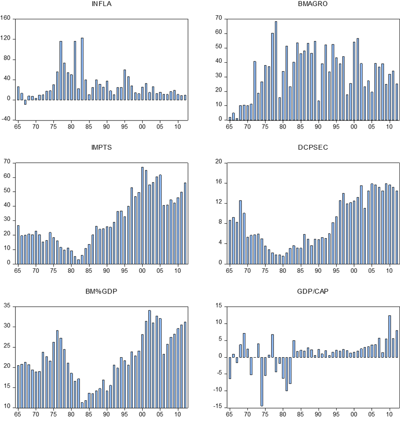
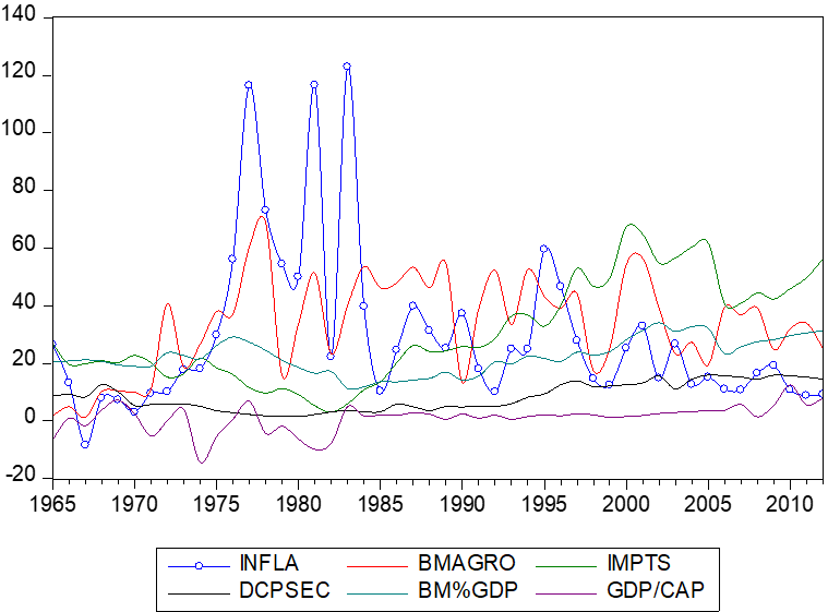
The study started with a pictorial representation of the behavour of variables over time. This helps to get a clearer view of the behavour of these variables involved and do a trend analysis just at a glace

INDICATOR	Mean(%ave)	Std Dev.	Minimum	Maximum
INFL	29.3	28.4	-8.4	122.9
BMGR	33.7	16.7	1.23	68.5
IMPTS	30.7	17.7	3.0	67.2
DCPS	8.4	4.9	1.5	15.9
BMG/GDP	22.4	60	11.3	34.1
GDP/CAP	1.1	4.7	-14.5	12.4

Source: Author’s Calculations. WDI, 2017 Data Base, from 1965-2012.

Inflationary pressure were experienced in the economy in the 1970s and the 1980s. Where inflation figures reached their peak as 116% in 1977 and 1981, the worst inflationary figures record was in the 1983, where inflation peaked at 122.9%, this could be as a results of the wild fires that destroyed the large track of forest and the agricultural base of the economy of Ghana. This period was also characterized with much government interventions in the market, lots of restrictions imposed on commercial banks, coupled with large public sector borrowing; which reduced market capitalization and private sector investment mainly as result of high political instability in the economy. Actual output levels fell far below the potential, creating highly unbearable inflationary pressures in the economy, right after the economy recorded a negative rate of -8.4 inflation in 1967 as a results of the industrial drive embarked upon by the state which reduced imports and increased national outputs levels.

Broad Money Growth exhibited a study increase and peaked from 1977 upward with annual average of 33.7%, and the minimum figure recorded was 1.23% and maximum 68.5% annual growth rate. The Domestic Credit to the Private Sector equally exhibited some positive trends averaging annually at 8.4% and peaking at 15.9% annually. This could be as a results of the pre-1998 financial reforms and the financial sector adjustment programme (FINSAP) in the 1988, which resulted in an increase of commercial banks and non-banking institutions significantly across the country.

Imports  of Goods and Services has continued on an increasing trend until 1975 to 1980 where import figures begun to exhibit a declining trend in the economy; and has since taken an upward trend averaging annually at 30.7% with the minimum of 3.0% and maximum 67.2%, between 1982 -1985, while GDP Per Capital growth rate  took  sharp fluctuation between positive and negative figures from 1983 – 1984, with  highest negative value recorded ever was -15% in 1973/74; this phenomenon could be attributed to the high political instability  which discouraged private sector investment in the economy, coupled with the wild fires that destroyed many cocoa farm lands across the country.

This variable took an upward trend from 1985 and still continuing on that path, peaking 12.2% in 2010. GDP Per Capita was used for the trend analysis and empirical estimation due to its ability to measure the consumer welfare almost at the household levels in the economy.

The rest of this paper is organized as follows; section 2, reviews the related literature, section 3, the methodological framework and the analysis of the empirical results respectively, while section 5, looks at summary of major finding, conclusion and policy implications of the study, and finally, the references for the study.

2. Review of Related Literature

2.1. Theoretical Literature Framework

2.2. The Demand for Money

The amount of money consumers would like to hold in easily convertible form, such as liquid cash, and bank deposits is represented in the form:

Md =P*L(R, Y)………………………………………………………………………………………..…1

Where P, is the price levels, ‘R’ is the market rate of interest and ‘Y’, the income level. L(R, Y), the liquidity preference, desire to hold liquid cash instead of putting them in interest bearing assets. From the Portfolio Theory of Money Demand, Md = L (+Y, -R).

2.3. The Quantity Theory of Money and the Money Multiplier

The quantity theory of money postulates that money supply and price levels in an economy are in direct proportion to each other, a change in money supply brings a proportionate change in price levels. Mostly represented by the Fisher Equation in the form:

M*V = P*T………………………………………………………………………………………………2

Where M, is, Broad Money, M2, V is Money Velocity, V= ,the average number of times a cedi is spent per year, P, is the general price Level and T, Volume of Transaction or the output levels in the economy, and Ms, the Money Supply.

 In a growth model, the above equation assumes the form;

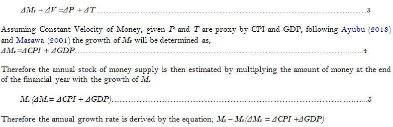
For reserve money programme requirement, a monthly growth rate is attained by dividing the annual rate by 12. The monthly stock of money supply is derived by adding the stock of M2 at the closing of the current year with the calculated monthly growth rate.

To control the quantity of money, excess money supply, or the idle money balances in the economy, the central bank often times adopts  measures such as the ‘‘The Reserve Money Programme’’ on the assumption that the relationship between money supply and the monetary base is constant; implying:

Where, M2 is the Broad Money Supply, MO, is the Base Money, and ‘λ’ is the Money Multiplier. A change in the Money Supply is brought about as a result of a change in either monetary base, Mo or the Money Multiplier, λ.

Central bank base money, Mo is made up of either central bank’s source assets or liabilities; the assets include Net Foreign Assets (NFA), Net Domestic Credit (NDC), and Other Items Net (OIN), Ayubu (2013). This implies:

While the liabilities incorporate the commercial banks deposits at the central bank and currency in circulation.

2.4. The Money Multiplier, λ,

This refers to  the amount of money that commercial banks are able to generate with each dollar of their reserves (the amount of deposits the central banks requires commercial banks to hold on and not lend.) takes the form;

Where λ is the Money Multiplier, c denotes currency in circulation, d is the demand deposits, err, the excess reserves and rr is the required reserve ratio (Ayubu, 2013; Masawa, 2001). Though Monetarism has been criticized by Kenyans school of thought, it has been widely accepted and used to control inflation on the market by the monetary authorities in many economies.

2.5. Theoretical Inflation Model

Inflation, a persistence rise in the general price level of goods and services in the economy, is modelled following Ubide (1995), Moser (1995), Adu and Marbuah (2011), Laryea and Sumaila (2001), Akinboade et al. (2004) and Ayubu (2013) and Masawa (2001) According to the mentioned previous papers, inflation in an open developing economy is assumed to be theoretically derived from weighted average prices of tradable ( Pt ) and non- tradable goods( Pnt );

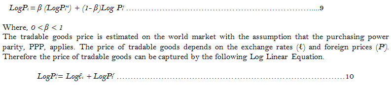
Economic theory stipulates that both exchange rate appreciation and decrease of foreign prices will lead to a decline of domestic prices. On the other hand, the depreciation of the exchange rate and increase in the foreign prices increase the domestic prices and that there is a parallel movement between the overall demand of the country and demand for non-tradable goods. Given that the overall demand is determined by real money balances, it is therefore assumed that prices of non-tradable goods is determined by real money balances, which defines the equilibrium condition in the money market; where Real Money Demand,( md ), equals Real Money Supply,( ms ), this equation assumes the form;

Where mtd is the Real Money Demand, msd, is Real Money Supply and ɸ, is a scale factor representing the correlation between the aggregate demand and demand for non-tradable commodities in an economy and  again, Real Income, Interest Rate and Inflationary Expectation are assumed to determine Real Demand for Money among consumers;

Where, mtd, is the demand for real idle money balances, yt, real income, rt nominal interest rate and πt, expected rate of inflation. From economic theory, the partial derivatives, real income, inflation and demand for idle money balances is positive, while interest rate is rather negative; all thing being equal.

Guided by Moser (1995) and Ayubu (2013) the Adaptive Expectation model estimates the inflation expectation model as specified below.

Where ΔLogρt-1), and   πt-1 represent inflation and expected respectively in both period, t-1. Normalizing d1 = 1 for simplicity in the derivative procedure, and substituting it into Equation 13 and rearranging, yields the log linear form of Equation 14 as below.

Notwithstanding the above log linear model, Ubide (1995) and Ayubu (2013) advanced the argument of the inappropriateness of using the interest rate, as a financial measure to measure domestic opportunity cost in countries with less developed financial sector such as the experiences in the LDCs.

2.6. The Structuralist and Keynesian Theory

The Structuralist argues that by the very nature of their economies, LDCs are prone to inflation as most of them are characterized by structural rigidities, unproductive government interventions, and political interferences in these economies. While the Keynesians argue also that organized labour pressures on government pushes wages up, and  when not matched with output levels creates inflationary pressures; and most of these LDCs are net importers of energy and most industrial imputes and other basic necessities of life.

The choice of variable for this study, in addition to economic theory, followed  Diouf (2007), Drevall and Ndung’u (2001) and Yen, Xie, Yuan, and Cui (2015) etc. and  used variables including Broad Money Supply, Imports of Goods and Services, Domestic Credit to the Private Sector,  and Gross Domestic Product Per Capita.

2.7. Empirical Literature Review

Inflation has been a major economic variables that researchers have kept close eyes on and continue to explore due to its direct or indirect effect on other socioeconomic factors in most countries, including Ghana. The period 1957-1972 is classified as the first episode of inflationary situation in Ghana, which was marked by active involvement of the state in the economic activities of the country where almost all industrial setups were undertaken by the government; inflationary pressures peaked from 1973-1982, as this period was marked series of military interventions and most of the agricultural base was destroyed by wild fires all across the country .From then, several economic policy interventions have been introduced by successive governments to keep inflation under control either through monetary policy (interest rate and money supply) or fiscal policy (Taxes and government expenditure).

Notwithstanding, it appears the efficacy of any these policy tools have not manifested enough on the inflation dynamics in the economy over the years; this has left policy makers and economists wonder whether inflation targeting is the way to go as has been experienced in the economy over the years. Government fiscal policy, as argued by different schools of thought, that this particular policy tool is highly influenced by political considerations, rather than economic principles in the country.

Numerous empirical studies have been conducted in both developed and developing economies across the world of which this section tries to explore some of these empirical studies on the subject matter under discussion for this paper.

Inflation in Ghana has also been extensively researched into from both monetary side and real side of the economy.

A study conducted by Lawson (1966) noted that the major contributory factor to the process was deficit incurred on government accounts and which were financed through borrowing from the domestic banking systems. This assertion confirms the monetarist’s hypothesis. The study also posits that inflation was further strengthened by the shortage of essential consumer goods and restrictions of imports which have aborted as a results of structural rigidities in the country.

Ahmed (1970) study from 1960-1965 confirms Lawson’s study over the same period. Ahmed (1970) also noted that excessive monetary expansion rising from government borrowing from the banking sector to finance budget deficits generated strong inflationary pressures in the economy.

Kwakye (1981) works also established that deficiency in local food production procedures is a contributing factor to the general inflation pressures. This also can confirm further results of various studies on  Ghana’s inflation as well as the Structuralist paradigm that food supply constraints plays a major role in price inflation in LDCs. He argued, this could be blamed on the increasing demand on agricultural production resulting from growth in the population and urbanization. That productivity growth is always met with structural rigidities, and so growth does not match with increase in population; excess demand for food results in significant price increases see (Gyebi & Boafo, 2013).

Many economic research papers have showed that fundamental macroeconomic indicators such as inflation and fiscal deficit play a very significant role in the high interest rate spread in Ghana. Bawumia (2003) using firm and market specific factors revealed that factors including lending risk, public sector borrowing, low savings rate, inflation and exchange rate play a critical role in the systemic rise of interest rate in Ghana.

Adu and Marbuah (2011) also confirmed the nexus between inflation and interest rate and other macroeconomic determinants in Ghana; using data from 1960 – 2009. This paper concluded that the positive inflation-interest rate nexus is due to the short term interest rate being a principal policy anchor in inflation targeting framework of the central bank of Ghana. Other studies examines the rapid exchange rate depreciation and the resultant hikes in import prices are in themselves inflationary, hence cannot be ignored in explaining the changes in interest rate in Ghana.

Sowa and Kwakye (1993) felt there were other factors that could more explain the inflationary dynamics in Ghana other than just monetary elements, as the results of some studies have shown. Sowa and Kwakyi argued that proxying the real side as monetary factor in inflation models does not allow for the clear isolation of the real side of the economy; and so decided to do an econometric modelling using all possible source of inflationary pressures, it came out that monetary growth and exchange rate were significantly contributing to inflationary pressures in the Ghanaian economy also see (Gyebi & Boafo, 2013).

Most empirical studies on inflation in the Ghana’s economy have indicated money supply as playing a significant role in price movements in the economy. Example, works of Lawson (1966); Ahmed (1970); Ewusi (1977) and Kwakye (1981) attributed the inflationary pressures to excessive monetary expansion which results from government borrowing from the banking sector for deficit financing.

Growth in nominal GDP was used as a proxy for real output represented by (Y) in Gyebi and Boafo (2013) modelling of the Ghana‘s inflation. Their study posits that in the  Ghanaian economy, output is determined by the expenditure approach and the government has traditionally been a major consumer of non-productive items and  that a rise in output would mostly induce inflation in Ghana, and argued that large spending on central government protocol services, travelling abroad, conduction of general  elections and supplementary elections and national security do not increase the supply of real goods in the economy, this according to the study, will result in an increase in aggregate demand over aggregate supply, and hence, trigger inflationary pressures in the local economy (Gyebi & Boafo, 2013).

Us (2004) conducted his study using data from 1990-2002, on Mo and inflation figures in Turkey, and concluded that there is no any significant relationship between these variables, according to the study. Also he used data on M1, M2 and M3 in the Euro Area from 1990-1997, and find a positive and significant relationship between the variables used and the inflation. Diouf (2007) used variables on Broad Money from Mali between1979-2006, and discovered a significant long and short run relationship between these monetary variable and inflation. Pindiriri (2012) conducted his study in Zimbabwe, using monthly inflation data and M3 from 2009-2011 and found a positive and significant relationship between variables used for the inflation model.

Darrat (1986) did his study using M0, in North Africa, 1960-980 quarterly data, it was revealed that there is a Positive relationship between these variables and inflation dynamics; Thornton and Ocasio (2008) used Money in circulation, M1 and M2 from African economies between, 1960-2007 and concluded that there is a Weak relationship between variables for counties with inflation and money growth below 10%.

Drevall and Ndung’u (2001) used data on M1&M2 from Kenya between, 1974 – 1996 and concluded that the relation that one can conclude exists between these variables is only in the short run, and there is no significant relationship in the long run; Simwaka, Ligoya, Kabango, and Chikonda (2012) did their study on inflation and M2 in Malawi using Monthly data from 1995 -2007 and came to the conclusion that there exists a Positive relationship between these variables.

Morana and Bagliano (2007) based their study on M1, M2, and M3 in the USA from 1959 – 2003, the study established a Positive long run relationship among variables used for their estimation; Kabundi (2012) used M3 on Ugandan Monthly monetary data from 1991-2011 and was able to establish a Positive and significant relationship between inflation and M3. Akinboade et al. (2004) also based his studies on inflation and  M1 & M2 in Nigeria using time series data between 1986 -2008 and found a  Positive and significant relationship between these series; Zhang (2012) conducted a study also using a time series data on M2  in China from  1980 -2010 and also concluded on a  Positive relationship between the series .

Drevall and Ndung’u (2001) conducted a study on inflationary processes in Brazil from 1968 - 1985, it was revealed that the degree of inertia, as indicated by the coefficient value of the lagged inflation was 0.41 and also established that an increase in money growth and oil prices also has a positive impact on inflation in Brazil.

3. Methodology and Estimation Strategy

3.1. Model Specification and Data

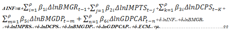
Following Lim and Sek (2015), Drevall and Ndung’u (2001), Diouf (2007)  and  Ayubu (2013) the equation below is specified in this study, to help do  an empirical exploration of the inflation determinants in Ghana, and its relationship with the Friedman’s theory on inflation.

INF =ƒ(BMG, IMPTS, DCPS, BM/GDP, & GDP/CAP)………………………………………15

Where INF, is inflation, BMG, is the Broad Money Growth, DCPS, is Domestic Credit to the Private Sector, Broad Money % of GDP, and GDP Per Capita.
Equation 15 can be transformed into an econometrics model as natural logarithm is applied to obtain a linear exponential trend, if any, in this time series data for this study.

INFt = β0+β1LnBMGRt + β2LnIMPTSt + β3 LnDCPSt + β4 LnBM/GDPt + β5GDP/CAPt + µr ……………………………………………………………………………………………………………………………………………………………………………………………………………………………………………...16a

Where the coefficients; βi, ( i = 1, 2 ……………5) , the estimated parameters /coefficients of the variables in the model specified and β0 , is the constant term while t, the time variant nature of the variables in the model specified. Ln, represents the natural logarithm used to transform the equation for its exponential trend and, µ the error term, the Log-log transformation was not applied to Inflation and GDP Per Capita, as there are negative values involved in the data series of these particular variables, though their log transformation do not affect the statistical values generated and their inferences from the data set.

3.2. Data Source

Annual time series data (a set of observations collected at usually discrete and equally spaced time interval) on Ghana’s economy was sourced from World Bank, World Development Indicators, (WDI) 2013 for all variables used for this study, from 1965 -2012

3.3. Definition of Variables and a Priori Expectation

Inflation ; this refers to the persistent increase the general price level of goods and services in the economy; in this study the CPI was used as an endogenous indicator for the estimation as this has direct bearing on the average wellbeing of the consumer/household in the economy.

Broad Money Growth, M2, this is the monetary aggregate, is a measure of the money stock that include M1(currency and coins held by the non-bank public, checkable deposits, etc. ) plus savings deposit including money market deposit accounts, short-term time deposits in banks etc.

The coefficient of this variable, is expected to have a positive relationship, β1 ˃ 0, with inflation variable, see Zhang (2012); Akinboade et al. (2004); Drevall and Ndung’u (2001). From Friedman’s Quantity Theory of Money; an increase in monetary growth will increases general price levels, but does not really affect output levels in the economy, Friedman (1963).

Imports of Goods and Services, a leakage, according to the aggregate demand theory, when the price level is higher, the real GDP demanded is low. One of the explanations given is that, this is an illustration of the consequence of the Mundel-Fleming model. As the price levels drops, interest rate falls, investment in foreign economies increases, the real exchange rate depreciates, net exports increases and aggregate demand increases; suggesting that increases inflation means more imports and less exports. However, increased inflation should also increase the exchange rate ie, currency depreciates, in an economy where agents can trade foreign currency  for more domestic currency, then exports should increase and imports rather decreasing, all thing being equal, 0˂ β2 orβ2 ˃ 0 . Therefore the coefficient signing of this particular exogenous variable is indeterminate a prori.

Domestic Credit to the Private Sector , this refers to financial resources provided to the private sector (Investment Agents) by financial intermediaries, such as through loanable funds, purchase of nonequity securities and trade credits and other accounts receivable, that establish a claim for payment. This is expected to increase market capitalization or capital accumulation in the economy in general. The expected signing of the coefficient of this particular variable is negative, 0 ˂β3 , in that as loanable fund theory postulates, market capitalization increases with output levels, reducing the general price levels of goods and services in the economy. However, in an open economy where there is high level capital flight, market rigidities, and high level political interferences in the economy, an increase in credit to the private sector, will increase general price levels, as these increase may not reflect in the domestic economic out, making β3 ˃ 0. Again, the signing of this variable is indeterminate a prori.

Broad Money as a Percentage of GDP, Broad Money to GDP ratio reflects the very breathe of financial market, financial deepening or an aspect of financial development in an economy. However, this does not entirely or appropriately capture access to finance, financial intermediation or market capitalization. This variable is expected to be signed positive,β4 ˃ 0, as an increase in the percentage ratios, increases inflation in the economy, as it equally increases idle money balances in the hands of consumers/households.

GDP Per Capita Growth, is the Gross Domestic Product divided by mid-year population. Per Capital GDP is a measure that accounts for the consumers/household and the total population, making it a desirable parameter to measure economic wellbeing of agents. In a healthy economy with low level of unemployment and higher wages; there is an increase in the purchasing power of households, leading to an increased demand for goods and services, which feeds into the general price levels. A decrease in purchasing power, decrease demand for goods and services, leading to a decrease in production levels, reducing GDP and inflation. The prori expectation of β5 ˃ 0 a positive signing of this parameter.

3.4. Estimation Techniques

The stationary properties of the variables used in Equation 16, are examined. This is a necessary precondition for Cointegration analysis, and subsequent estimations of long-run and short-run results. This paper makes use of Augmented Dickey-Fuller (ADF); (Dickey & Fuller, 1979) and the nonparametric Philips-Perron (PP), which helps to ascertain the robustness of the stationarity test procedures involved in the study with time series data, Philips and Perron (1988). The null hypothesis of unit root, hence non-stationarity is examined against the alternative hypothesis of no unit root, implying stationarity.

The test is done with both a constant but no trend and with constant and trend. Again, the test is done at both the levels and first difference. Investigating stationarity properties of variables is necessary to avoid estimating a spurious regression for this stuy.

4. Empirical Results and Discussion

4.1. Estimation Technique

The estimable Econometric Model in Log-Linear form in Equation 15, is below;

LnINFt = β0+β1LnBMGt + β2LnIMPTSt + β3 LnDCPSt + β4 LnBM/GDPt + β5 LnGDP/CAPt +µr……………………………………………………………………………………………………...16b

This represents the long-run equilibrium relationship, where; βi, ( i = 1, 2 ……………5) represent the elasticity coefficients, and β0 , is the constant term while t, the time variant nature of the variables in the model specified. Ln, represents the natural logarithm used to transform the equation for its exponential trend and, µ the error term. The idea of avoiding a log transformation of negative values is more grounded in Mathematics, than in Economics and Statistics, especially, when large volumes of positive whole numbers are involves in the data series, statistical inferences are largely not affected.

All variables to be estimated are in natural logarithm. The choice of the log-linear model was based on the premise that log transformation allows the regression model to estimate the percentage change in the dependent variable resulting from the percentage change in the independent variable; log-log estimations also help to reduce the problem of Hetroschedasticity as it reduces the scale in which the variables are measured from a tenfold to a twofold (Gujarati, 2004).

The model was estimated using the Autoregression Distributed Lag (ARDL) framework also known as the Bounds Test. The testing procedure of the ARDL is performed in three steps. First, the Ordinary Least Square (OLS) is applied to an Error Correction Model (ECM), to test for the existence of a Long-Run relationship among the variables by conducting the F-Test for the joint Significance of the coefficients lagged levels of the variables.

Once the existence of Cointegration among the series is established, the second step involves establishing the coefficients of the long run relationship and making statistical inferences about their values, Pesaran, Shin, and Smith (2001). The final step involves estimating an Error Correction Model to obtain the Short-Run Dynamics in the parameters. The ECM generally provides the means of reconciling the short-run behavour of an economic variables with its long-run behavour.

4.2. ADF and PP Test for Unit Root (A Residual-Based Test)

Prior to testing for the existence of long-run level relationships (Cointegration) and estimating the corresponding Cointegration Vector (CV) and the Dynamic Error Correction Model (ECM) the order of integration of the individual series were examined using Augmented Dickey-Fuller, and Philips-Perron Test for unit roots was done to help determine the stationarity or otherwise and the order of integration in the series. The Engel-Granger and Philips-Perron residual based tests for Cointegration are simply unit root tests applied to the residuals obtained from SOLS estimations, under the assumption that the series are not cointegrated, all linear combinations of  (yt , Xt/ ), including the residuals for the SOLS, are unit root nonstationary. Therefore a test of the null hypothesis of no Cointegration against the alternative of Cointegration corresponds to a unit root test of the null of nonstationarity against the alternative of stationarity.

The study begun the analysis by estimating the unit root test proposed by Dickey and Fuller (1979) and Philips-Perron methodology proposed for time series data analysis. The two test differ in the method of accounting for serial correlation in the residual series; the Engel-Granger test uses a parametric Augmented Dickey-Fuller approach, while the Philips-Perron test uses the nonparametric  Methodology.

4.3. ADF Test for Unit Root

The Engel-Granger test estimates ρ-lag augmented regression of the form;

The number of lagged differences ρ should increase to infinity with the (zero-lag) sample size but at a rate slower than T 1/3 .  Study considered the two standard ADF test statistic one based on the t-statistic for testing the null hypothesis of nonstationarity, (ρ = 1) and the other based directly on the normalized

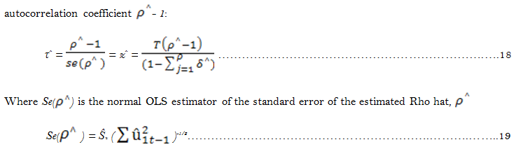
4.4. PP-Test for Unit Root

Contrary to the ADF Test proposed by Engel-Granger for Cointegration test, the PP-Test, a nonparametric test, obtains an estimate of Rho (ρ) by running the unaugmented Dickey-Fuller Regression in the form;

Δȗ1t = (ρ-1)û1t-1+ ωt.....................................................................................................................................20

And using the results to compute estimates of the long-run variances, ωw and the strict one-sided long-run variances λ1w of the residuals. The biased corrected autocorrelation coefficient is then given by the equation below with both T-Statistic and Z-Statistic.

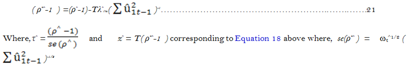
For ADF and PP statistics, the asymptotic distributions of the Engel-Granger and Philips-Quliaris Z and T statistics are nonstandard and depend on the deterministic regressors’ specification, so the critical values for the statistics are obtained from simulation results. In addition, the critical values for ADF and PP test statistic must accounts for the fact that the residuals used in the tests depend on the estimated coefficients of the model specified.

Accepting the null hypothesis implies () does not granger-cause (). Hence the exogenous variable (Inflation rate, Broad Money Growth, Imports of Goods and Services Domestic Credit to the Private Sector, Broad Money as a Percentage of GDP and GDP Per capita) cannot predict the future values of Inflation.

The test for unit root and existence of Cointegration in the data series was done using ADF and PP procedures at the levels with intercepts and trends. The results presented in the table below.

The results as obtained from the Eviews 10.0, revealed a mixed stationarity properties as can be observed from the table. While some variable are integrated of order one I(1) some are integrated of order zero, I(0). Implying that some of the variables exhibit stationarity properties at the levels, while other became stationary after first differencing. The mixed I(0) and I(1) properties was revealed regardless of the test procedure(ADF) or (PP) employed; as well as , whether the test is with intercept and trend.

All variables, after first differencing, exhibiting stationarity properties, strongly rejecting the zero null hypothesis of a unit root. This implies that a shock to any of the variables is likely to be temporal; since the variables are mean reverting, at most after first differencing, and so any estimate  will not produce any spurious results from the series (Abeberese, 2017).

VARIABLES	ADF-TEST		PP-TEST
Panel A:Levels	Constant	Constant&Trend	Constant	Constant&Trend
INFLA	t-stat [-2.4223] prob(0.1413 )	t-stat [-4.2790] prob(0.0074 )**	t-stat [-4.300] prob(0.001)**	t-stat [-4.3466] prob(0.006 )**
LN BMGR	t-stat [-4.3575] prob(0.001 )**	t-stat [-4.338] prob(0.0063 )**	t-stat [-4.273] prob(0.001 )**	t-stat [-4.2769] prob(0.007 )**
LN IMPTS	t-stat [-0.6778] prob( 0.8423 )	t-stat [-2.4885] prob(0.3320 )	t-stat [-0.7313] prob(0.8287 )	t-stat [-2.293] prob(  0.4294)
LN DCPS	t-stat [-0.844] prob(0.7970 )	t-stat [-2.105] prob(0.5296 )	t-stat [-0.772] prob( 0.8177)	t-stat [-1.973] prob( 0.6008)
LN  BM/GDP	t-stat [ -1.175] prob(0.6772 )	t-stat [-1.7214] prob(0.7259 )	t-stat [-1.3273] prob(0.6092 )	t-stat [-1.8634] prob( 0.6574)
GDP/CAP	t-stat [-4.457] prob(0.008)**	t-stat [-5.273] prob( 0.000)***	t-stat [-4.473] prob(0.000)***	t-stat [-5.263] prob( 0.000)***
Panel B: 1STDifference	Constant	Constant&Trend	Constant	Constant&Trend
ΔINFLA	t-stat [-11.980] prob(0.000 )***	t-stat [-11.884] prob(0.000)***	t-stat [-14.235] prob(0.000 )***	t-stat [-16.2417] prob(0.000 )***
ΔLNBMGR	t-stat [-8.640] prob(0.000 )***	t-stat [-8.821] prob(0.000 )***	t-stat [-13.925] prob(0.000 )***	t-stat [-12.929] prob(0.000)***
ΔLNIMPTS	t-stat [-3.202] prob(0.000 )***	t-stat [-3.223] prob(0.000)***	t-stat [-6.356] prob(0.000 )***	t-stat [-6.336 ] prob(0.000 )***
ΔLNDCPS	t-stat [-7.496] prob(0.000 )***	t-stat [-7.631] prob(0.000 )***	t-stat [ -7.504] prob(0.000)***	t-stat [-7.825] prob(0.000 )***
ΔLNBM/GDP	t-stat [  -6.450] prob(0.000 )***	t-stat [ -6.442] prob(0.000)***	t-stat [- 6.4513] prob(0.000 )***	t-stat [-6.442 ] prob(0.000 )***
ΔGDP/CAP	t-stat [-5.047] prob( 0.000)***	t-stat [ -5.276] prob(0.000)***	t-stat [-26.364] prob(0.000)***	t-stat [-28.770] prob(0.000)***

Note: *,**,***, denotes the rejection of the null hypothesis of unit root at the 10%, 5% and 1% significance levels respectively. The critical values for the ADF and PP tests statistics are -4.165, -3.508, -3.184, and at the 1%, 5% and 10% significance levels respectively. Δ is the first difference operator. The lag length selection for the Phillips-Perron test is based on Newey-West. Results were obtained from Eviews 10.0 Econometric software.

After conducting the unit root test, Inflation was revealed that inflation variable was not stationary at the levels as its probability value was not significant at 1%, 5% and 10% significant levels. But became stationary when trend and intercept were added to the equation even with both ADF and PP procedures. On the contrary, Broad Money Growth was significant at 5% significant level; implying stationarity at both Levels, Intercept and Trend with both ADF and PP estimation procedures. Indicating a pure I(0) variable.

The Imports of Goods and Services and Domestic Credit to the Private Sector Variables were not significant at all levels of significant (1%, 5% and 10%) irrespective of the test procedure used (ADF or PP) here, and whether with Intercept and Trend, however, they all became significant, attaining stationarity, after first differencing at all significant levels; exhibiting an I(1) property in the series. Meanwhile, Gross Domestic Product variable was significant at 1%, 5% and 10% significant level at the levels with both constant and trend, irrespective of the test procedure used.
The mixed stationarity properties exhibited in the series is suggestive of the use ARDD Framework for Cointegration test and subsequence of  the estimation of both long run and short run coefficients and Error Correction equations, as the framework accommodates  I(0), I(1) or a mixture of both I(0) or I(1) properties in time series data.

4.5. The ARDL Framework

The study adopts the Autoregressive Distributed Lag (ARDL) procedure, ie the Bound Testing Approach to Cointegration, proposed and popularized by Pesaran et al. (2001) to examine the dynamic of inflation determinants in Ghana. This framework has some econometric advantage over the Engel and Granger (1987) and the Maximum Likelihood Test based approach by Johansen and Juselius (1988). Cointegration techniques.

First, the Bounds Test does not requires pretesting of variables to determine their order of integrations since test can be conducted whether the series are I(0), I(1) or mutually integrated. Second, ARDL is efficient in the case of small and finite samples, the study can easily estimate the Long-Run Model by simply applying the ARDL methodology in the form:

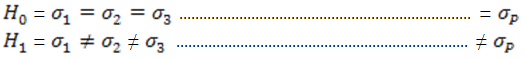
Whereμt is the disturbance term with zero mean and a finite variance, δ2, and ECMt-1 is the error correction term. From here, the study first uses the Wald-Test (F-Statistic) to test for the joint statistical significance of the coefficients of the lagged levels of the variables are statistically significant or not; hypothesizing that:

H0: δ1=δ2= δ3= δ4= δ5= δ6=0

H1: δ1 ≠δ2≠ δ3≠ δ4≠ δ5≠ δ6 ≠ 0

Given that the underlying series are a mixture of I (0) and I(1) processes, the study proceeded to test for the existence of Cointegration based on the ARDL framework, using the F-Bound testing approach for the joint statistical significance of the lagged levels coefficients. The results of the Cointegration test are presented below.

4.5.1. Results of Bound Test for Cointegration

EC=INF-( 1.0172*BMGR-0.3304*IMPTS-1.497*DCPS+1.74*BMGDP-19.89 )
F-Bound Test	Null Hypothesis: No Levels Relationship
Test-Statistic	Value	Significance	I(0)	I(1)
Calculated F-Statistic =	11.553	10%	2.08	3.0
K =	5	5%	2.39	3.38
Actual Sample Size	47	1%	3.06	4.15

Note: Results obtained from Eviews Econometrics software 10.0.

From the table above, the calculated F-statistic, 11.553 is greater than the upper bound values at both 10%, 5% and 1% significance level. Since the F-statistic is greater than the upper bound values at all significance level, the zero null hypothesis of No Levels Relation is strongly rejected.

Therefore there is a long-run relationship among the data series when inflation is normalized on the regressors. The test will have been inconclusive, if the F-statistic value fell between the lower bound and the upper bound, or have no cause to reject the Null hypothesis, if F-statistic fell below the lower bound. With the existence of Cointegration established, the study can now go ahead and estimate the Long-Run coefficients of the relationships

4.5.2. The Long–Run Relationship Equation

DPNT VARIABLE(INFt-1)		ARDL(1,1,1,1,1), Selected Based on SIC, AIC,HQ
Variables	Coefficients	Standard Error	T-Statistics	P-Values
Constant	-19.376	13.652	-1.419	0.1646
INF*(t-1)	-0.9756***	0.1163	-8.3903	0.0000
LnBMGR(t-1)	0.99237***	0.2607	3.9591	0.0000
LnIMPTS(t-1)	-0.322	0.3737	-0.863	0.3943
Ln DCPS(t-1)	-1.461	1.4229	-1.026	0.3116
LnBM%GDP(t-1)	1.6994*	0.6399	2.656	0.0118
LnGDP/CAP(t-1)	-1.658*	0.9050	-1.832	0.0755

Source: Author’s Drawing; World Bank Data (WDI: 1965-2012). Note: *, **, ***, denotes the rejection of the null hypothesis of; βi, ( i = 1, 2 ……………5) = 0, at the 10%, 5% and 1% significance levels respectively. Results obtained from Eviews 10.0 Econometrics software.

4.5.3. The Short-Run Dynamic Equation

The Long-Run equation can be reparametarized and expressed into an Error Correction Model:

DPDNT VARIABLE(INFt-1)		ARDL(1,1,1,1,1), Selected Based on SIC, AIC,HQ
Variables	Coefficient	Standard Error	T-Statistic	P-Values
DLn(BMGR)	0.997***	0.1406	7.094	0.0000
DLn(IMPTS)	0.952*	0.408	2.331	0.0256
DLn(DCPS)	-0.776	1.346	-0.577	0.5679
DLn(BM%GDP)	-5.193***	0.929	-5.593	0.0000
DLn(GDP/CAP)	0.7997*	0.472	1.693	0.099
ECM(Eqn)	-0.976***	0.100	-9.725	0.0000
R2	0.782

Source: Author’s Drawing; World Bank Data (WDI: 1965-2012). Note: *, **, ***, denotes the rejection of the null hypothesis of; βi, ( i = 1, 2 ……………5) = 0, at the 10%, 5% and 1% significance levels respectively. Results obtained from Eviews 10.0 Econometrics software.

4.5.4. Interpretation of Coefficients

The coefficients of the variable of interest for this study, Broad Money Growth (BMGR) and Broad Money as Percentage of GDP (BM%GDP) expectation were met, lending much credence to Friedman’s Monetary Theory. *** and *** were correctly signed (positive) in line with economic theory; The estimation revealed that a unit (1) increase in Broad Money Growth brings about 100 units increase in inflationary pressures in the economy in  the long-run, and this was statistically significant at 1% error level, according to the data used for this study. Absolutely supporting the monetarists’ theory on inflation. This phenomenon could be as a result of increase in liquidity preference, the desire to hold idle balances in the Long-Run, instead of keeping them in interest bearing assets by the economic agents; a possible cause of demand pull-inflation. Friedman posits that the role of governments and the central banks is to control the quantum of money in circulation in the economy, the theory asserts that variations in monetary growth has a significant impact on the national output (Y) in the short-run, and general price levels in the long-rum.

Contrary to the Long-Run relationship established; the Short-Run dynamics from the study rather revealed an inverse relationship between the inflation and Broad Money Growth variables. It came up from the estimation that a unit increase in Broad Money Growth, in the Short-Run will rather reduce inflationary pressures by 5 unit; implying that in the short-run, demand for idle balances is declines; agent will prefer investing any additional liquidity for economic gains, increased market capitalization engenders output growth and lowers inflationary pressures; however, from this study, further increases in Money Growth could have a deteriorating effect on the macroeconomic variables.   This findings is consistent with Lim and Sek (2015) who did similar studies using data from both advanced and developing economy and came up with such findings from their study.  Akinboade et al. (2004)  with data on Nigeria, and Drevall and Ndung’u (2001) Drewall and Ndung’u (2001) with data on Kenya, also got similar findings from their studies.  Morana and Bagliano (2007) studies on USA,   also corroborated this findings.

The coefficient of Imports of Goods and Services (IMPTS), (*) was appropriately signed to support economic theory. The Short-Run dynamics revealed that (* ) was positive and statistically significant at 10% significance level, implying that a unit increase in imports of good and service in the economy will increase inflationary pressures by 0.95 unit  in the economy; findings were consistent with Lim and Sek (2015). This phenomenon is mostly experienced in developing economies like Ghana, where the demand curve for imports of goods and service is price inelastic, a proportionate increase in import prices leads to less than a proportionate decrease in quantity demanded for imports. Ghana, a developing economy is a net importer of basic consumables, an economy where there is a high misconception about foreign products; unfortunately, foreign goods and services are associated with ‘good quality and affluence’ and local good are sometimes deemed as ‘inferior and poverty’ by economic agents, this is a misconception; as a results, any increase in idle balances in the hands of consumers/ household may lead to increase in imports of good and service in the Short-Run. However, this counter-productive economic behavour is reversed in the Long-Run; when the reality about foreign and national product become apparent.  From the estimation of the Long-Run relationship model; the estimated coefficient exhibited a negative relationship between imports and inflation, implying that agents begin to put their additional income into viable economic venture, though this coefficient was not statistically significant according to this study, however, this is an economically desirable revelation.

The coefficient of Domestic Credit to the Private Sector () was negatively signed, very consistent with economic theory of loanable fund and market capitalization. A unit increase in credit to the private sector lead to about 0.78 unit reduction in inflationary pressures in the economy in the Short-Run. And in the Long-Run, this leads to 100 units decrease in inflation; findings supporting (Mordi et al., 2007) on their studies of inflation in Nigeria. This phenomenon could be attributed to the Monetary Transmission Mechanism (MTM), where credit facilities to the private sector increases private investment and national output. This coefficient was not stat-sig, but a desirable economic revelation from this study on Ghana’s economy.

Another variable highlighted in this study was GDP Per Capita; the elasticity coefficient (*) was appropriately signed and the a priori expectation met; very consistent with economic theory; also statistically significant at 10% error level. The study revealed that a unit increase in GDP Per Capita variable lead to 0.8 unit reduction in general price levels in the Short-Run, but in the Long-Run, the reduction is estimated at 1.5 units. Implying that increases in the national output per capita level, makes supply out strips demand for goods and services; these makes more goods and services available to the consumer/household, subsequently leading lower prices of these products.

The R2, of 0.78, implies a very high explanatory power of the exogenous variables as used in the estimation of the model. Here, about 78% of the variations in inflationary pressures have been explained by the exogenous variables in the model.

The Error Correction Model (ECM) coefficient estimated was appropriately signed and statistically significant at 1% error level, further lending support to the Cointegration relationship among the data series. The implication here is that, inflation levels adjust at the rate of about 98% of the gap between its Long-Run levels and the current level in each period whenever there is a shock, in other words, about 98% percent of the deviations from an equilibrium path arising from the model is restored with a period of one year.

The Lag of Inflation (LnINFt-1), coefficient of -0.98, another important econometric revelation that about 98% of the previous period inflation is transmitted into the current period inflation, reflecting a strong ‘Backward Looking’ inflation expectation, E(πt) of consumers and the consumer behaviour in the Ghanaian economy; economic agents expect the future levels of inflation to be relatively close to what is was in the previous year.

4.5.5. Lag Length Selection

The information criteria are often used as a guide in model selection. There are many lag criteria for selection but in this study, the using the constant as endogenous variable and all other variables for the estimation of the lag length model, Final Predictor Error (FPE), Akaike Information Criterion (AIC), Schwarz Information Criteria (SIC), and Hannan-Quinun (HQ) all appeared significant in the selection criteria model used to determine the Autoregressive Distributed Lag Length, see Appendix II. Lim and Sek (2015) study on their inflation determinants, found that ARDL,(1,1,…..1) are mostly appropriate for inflation models in developing economies, while ARDL,(1,1, …0,0) are related to developed economies.

5. Summary of Major Findings

5.1. Some Descriptive Statistics from Trend Analysis

1. Ghana, in its economic history, recorded a negative inflation rate in 1967 at -8.4% with the highest inflation figures of 116% between 1977 -1981 and rose to 122.9% in 1983.
2. Broad money growth rate reached its peak, maximum, at 68.5% and the minimum growth rate of 1.2% per annum, with an annual average growth of 33.7%
3. Imports of goods and services increased marginally from 1965 upward and started to decline from 1975-1980, however, from 1981-1985, it begun to take a positive trend, averaging at 30.7% per annum, with the maximum growth rate of 67.2% and a minimum of 3.0% per annum.
4. Domestic credit to the private sector exhibited a sturdy increasing trend over the years, averaging annually at 8.4%, with the minimum recorded figure of 1.5% and 15.9% maximum. While  Broad money growth to GDP ratio equally exhibited a positive trend with annual average of 22.4%
5. Per Capita GDP growth rate have been fluctuating between both negative and positive values and this trend hit the trough at -15% in 1973-1974; and turning to positive values from 1985, reaching the peak in 2010 with maximum of 12.4%. However, the average annual growth rate over the period was 1.1% per annum.

The dynamic estimation technique employed in this study revealed a Cointegration relationship between the variables used in this empirical studies. Here, the elasticity coefficient of broad money growth exhibited a positive and significant relationship with inflation, both in the short dynamics and the long-run relationship. It was revealed that a unit increase in broad money growth brings about 100 units increase in inflationary pressures.

Again, the elasticity coefficient of the import variable in the model also exhibited a positive relationship with inflation in short-run dynamics; however, the long-run coefficient exhibited negative relationship with inflation. The study also revealed a negative relationship between domestic credit to the private sector both in the short and the long-run, but this elasticity coefficients were not stat-sig, according to the study. With Per Capita GDP growth rate, the estimates revealed an inverse relationship with inflation both in the short and long-run and this coefficient was statistically significant. Here, the degree of impact on inflation was stronger in the long-run than experienced in the short-run dynamics.

5.2. Conclusion

Inflation has been one of the major headaches of economic policy-makers in both advanced and developing economies. This paper set out to investigate the monetarists’ theory on inflation using the ARDL Bound-Testing framework with World Bank Data, WDI, 2017, with data spanning from 1965-2012 on Ghanaian economy. Conspicuously missing variables in this model are the interest rate and the exchange rate, as widely used in inflation determinants models. However, power structures and market rigidities do not allow these powerful macroeconomic policy instruments to exhibit their full economic effect on macroeconomic variables in most Developing economies, these interferences could make variables with such properties generate  a misleading estimates ill-suited for economic interpretations.

5.3. Policy Implications

High inflation rates induces uncertainties among economic agents and could have a deteriorating effect on the financial development and consumer budget, and can become a grave threat to macroeconomic and political stability in the economy, if not checked with appropriate policy tools. From the study it is evidently clear that the main objective of monetary policy will be best met by targeting monetary growth rate. The central Bank must formulate a monetary policy framework, critically targeting the growth of the monetary aggregate; this would have a strong positive impact on inflationary pressures both in the short and long run. The new central Bank Act, 2002, (Bank of Ghana Act, 612), must be strictly enforced to help grant total independence to the central bank so it can freely adopt the appropriate policy tool, to control excess liquidity on the market. Liquidity injection should target economically viable programmes rather than political consideration. An improved macroeconomic fundamentals is a prerequisite for economic, political and social stability of every economy.

5.4. Model Diagnostics Test Results

The diagnostic tests underlying the ARDL framework for Equation 16 were conducted for this study, these included, Granger-Causality Test, Correlogram Squared Residuals, Correlogram Q-Statistic, Jarque-Bera Test for Normality, and Recursive Test for Stability of the estimated model.

Granger –Causality Test: Correlation does not mean causation, the econometric graveyard is full of magnificent correlations which could be just spurious estimations; Granger Causality test measures precedence and information content in the model estimation but does not indicate causality. The study went further to test the variables which appeared significant in this model estimation searching for causality properties from these significant variables and results reported below. The Granger-Causality Test showed no bi-directional or unidirectional causality relationship between Broad Money Growth and Inflation variable, given their F-statistic and their P-values as [1.83114], (0.1829) respectively. See Appendix III.

Implying none of the variables granger causes the other, therefore the null hypothesis of no Granger-Causality cannot be rejected. However, Imports of Goods and Services to inflation and GDP Per Capita to Inflation variables exhibited a unidirectional causality relation, that is, from GDP Per Capita to Inflation, given their F-statistic [3.865], P-value (0.0614), though a weak causal relationship, here, we reject the null hypothesis of no causality relationship; implying the past values of GDP Per Capita could predict the future values of inflation.

With GDP Per Capita and Inflation the test revealed a Bidirectional causal relationship between these variables, from GDP Per Capita to Inflation and from Inflation to GDP Per Capita, with F-statistic of [5.090], P-value (0.0291) , and F-statistic [4.385], (0.003), here, the null hypothesis of no causal relationship is flatly rejected. Implying that the past values of each of the variables is good to predict the future values of the other.

The test also revealed that there is no causal relationship between imports and broad money growth variables, given their F-stat [0.094], (0.7604), and [0.003], (0.7604); as a results the null hypothesis of no causal relationship cannot be rejected, based on these statistics. However, GDP and Imports variables rather showed a bidirectional causal relationship with F-stat [4.331], (0.043), and [4.527], (0.0390). See Appendix; here, the null hypothesis of no causal relationship cannot be accepted. Implying that the past values of each of the variables is a good predictor of the future values of the other, according to the test.

The Correlogram Squared Residual, and Correlogram Q-Statistic Test showed no first order serial autocorrelation, given the large P-values, all greater than 0.05, making none of them stat-sig .see Appendix for diagnostics test results.

The Jarque-Bera Test statistic of [1.74], Prob. (0.419) for normality also failed to reject the null hypothesis that the residual errors are normally distributed. It came up that the residual errors in the estimated model are normally distributed, confirming that the errors are White Noise.

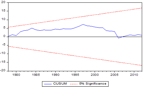
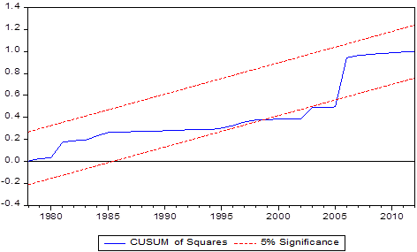
CUSUM and CUSUM-Square Test is estimated to determine the stability of the ARDL Models, a model exhibits stability if its recursive residuals is located within the two critical bounds, and this was found to be exactly so. However, the CUSUM-Squared test revealed some relative instability in some periods, which is, from the periods 1998-2002, and 2003-2006; and regained stability afterwards, see table below.

References

Abeberese, A. B. (2017). Electricity cost and firm performance: Evidence from India. Review of Economics and Statistics, 99(5), 839-852.

Adu, G., & Marbuah, G. (2011). Determinants of inflation in Ghana: An empirical investigation. South African Journal of Economics, 79(3), 251-269.

Ahmed, N. (1970). Deficit financing, inflation and capital formation. The Ghanaian Experience from 1960-1965, Munic Welerun Verlag.

Akinboade, A. O., Siebrits, K. F., & Niedermeier, W. E. (2004). The determination of inflation in South Africa: An econometric analysis. AERC Research Paper 143. African Economic Research Consortium.

Ayubu, V. S. (2013). Monetary policy and inflation dynamics. An empirical case study of Tanzanian economy: UMEA University, Sweden Press.

Bawumia, M. (2003). Monetary growth exchange rates and inflation in Ghana. An error correction analysis. Bank of Ghana Working Paper. W/P BoG-2003/03.

Darrat, F. A. (1986). Money inflation and causality in North African countries: An empirical investigation. Journal of Macroeconomics, 8(1), 87-103.

Dickey, D. A., & Fuller, W. A. (1979). Distribution of the estimators for autoregressive time series with a unit root. Journal of the American Statistical Association, 74(366), 427-431.

Diouf, A. M. (2007). Modelling inflation for Mali. IMF Working Paper, WP/07/295.

Drevall, D., & Ndung’u, S. N. (2001). A dynamic model of inflation for Kenya, 1974-1996. Journal of African Economics, 10(1), 92-125.

Engel, R. F., & Granger, C. W. (1987). Cointegration and error correction representation, estimation and testing. Econometric Society, 55(2), 251-276.

Ewusi, K. (1977). The determinants of price fluctuations in Ghana. ISSER Discussion Paper. Legon: University of Ghana.

Friedman, M. (1963). Inflation: Causes and consequences. New York: Asia Publishing House.

Gujarati, D. N. (2004). Basic econometrics (4th ed.). New York: McGraw Hill.

Gyebi, F., & Boafo, G. K. (2013). Macroeconomic determinants of inflation in Ghana from 1990–2009. International Journal of Business and Social Research, 3(6), 81-93.

Johansen, S., & Juselius, K. (1988). Hypothesis testing for cointegration vectors: With application to the demand for money in Denmark and Finland (No. 88-05).

Kabundi, A. (2012). Dynamics of inflation in Uganda. Working Paper Series No 152 African Development Bank.

Kwakye, J. K. (1981). An empirical analysis of price behaviour in Ghana. MSc Thesis University of Ghana. Legion. 

Laryea, S. A., & Sumaila, S. R. (2001). Determinant of inflation in Tanzania. CIM Working Paper. WP/12, Bergen.

Lawson, R. M. (1966). Inflation in the consumer market in Ghana. Economic Bulletin of Ghana, 10(1), 36-51.

Lim, Y. C., & Sek, S. K. (2015). An examination on the determinants of inflation. Journal of Economics, Business and Management, 3(7), 678-682.

Masawa, L. J. (2001). The monetary policy framework in Tanzania. Paper presented at the Bank of Tanzania Paper at the Conference of Monetary Policy in Africa, held in South Africa.

Morana, C., & Bagliano, F. C. (2007). Inflation and monetary dynamics in the USA: A quantity-theory approach. Applied Economics, 39(2), 229-244.

Mordi, C. N. O., Essien, E. A., Adenuga, A. O., Omanukwe, P. N., Ononugbo, M. C., Oguntade, A. A., . . . Ajao, O. M. (2007). The dynamics of inflation in Nigeria: Main report. Occasional Paper No. 2. Research and Statistics Department. Central Bank of Nigeria, Abuja.

Moser, G. G. (1995). The main determinants of inflation in Nigeria. IMF Staff Paper 270-287.

Pesaran, M. H., Shin, Y., & Smith, R. J. (2001). Bound-testing approach to the analysis of level relationships. Journal of Applied Economics, 16(3), 289-326.

Philips, P. C., & Perron, P. (1988). Testing for unit root in time series regression. Biometrica, 75(2), 335-346.

Pindiriri, C. (2012). Monetary reforms and inflation dynamics in Zimbabwe. International Research Journal of Finance and Economics, 90, 207-222.

Simwaka, K., Ligoya, P., Kabango, G., & Chikonda, M. (2012). Money supply and inflation in Malawi: An econometric investigation. Journal of Economics and International Finance, 4(2), 36-48.

Sowa, N., & Kwakye, J. (1993). Inflation trends and controls in Ghana. African Economic Research Consortium (AERC), Research Paper 22, Nairobi, Kenya.

Thornton, P. H., & Ocasio, W. (2008). Institutional logics. The Sage Handbook of Organizational Institutionalism, 840, 99-128.

Ubide, A. (1995). Determinants inflation in Mozambique. IMF Working Paper WP97/145.

Us, V. (2004). Inflation dynamics and monetary policy strategy: Some aspects for the Turkish economy. Journal of Policy Modelling, 26(2004), 1003-1013.

Yen, M. S. S., Xie, H., Yuan, P., & Cui, S. S. (2015). A study to examine the uses of personal strength in relation to mental health recovery in adults with serious mental illnesses: A research protocol. Health Psychology Research, 3(2).

Zhang, C. (2012). Monetary dynamics of inflation in China. World Economy. Available at: 10. 1111/twec/12021.