Influences of Monetary Policy Instruments on Domestic Investments and Economic Growth of Nigeria: 1970-2018

 

OKOROAFOR, O.K. David

Economics Department, University of Abuja, Nigeria.	Abstract This paper explores fertility preference and its associated factors among older Nigerian women within the reproductive ages 40 to 49. It considers the impact of proximate factors of place, wealth, education, use of contraceptives, and other associated factors on fertility preference. Using Nigeria Demographic and Health Survey (NDHS 2018) data, responses of 1357women of ages 40-49 years in the couples recode file were considered. Fertility preference is measured by “the desire for another child”. We use descriptive statistics and logistic regression to identify the associating factors and impacts of identified explanatory variables on the desire for another child. Result revealed up to 25% of women within ages 40-49 desire to have another child while 35% uses contraceptives. The desire by older women to have another child is higher in the rural areas than in urban areas while more than 50% with desire for another child have no education and are found practising Islam. Logistic regression result indicates that older women not using contraceptive have higher odd ratio with the desire for another child, those in urban areas have lower odd ratio while women in the Northeast and the Northwest have more than 2.5 chance of desiring for another child than those in the Southwest. This study concludes that the desire for pregnancy at later end of reproductive years must be controlled through women's education and community-based sensitization programs.
Licensed: This work is licensed under a Creative Commons Attribution 4.0 License.
Keywords: Private Economy Growth Influence Investment Money Domestic Policy. JEL Classification F3; E62; O16; G11.
Accepted: 20 April 2020 Published: 5 May 2020

Funding: This study received no specific financial support.

Competing Interests:The author declares that there are no conflicts of interests regarding the publication of this paper.

1. Introduction

Investment is perceived as boost for the attainment of an enduring economic development and poverty alleviation both in developed and developing economies. It magnifies entrepreneurship as well as create employment opportunities that brings about income for people in society. Investment in an economy is majorly fund driven. According to Tobias and Mambo (2012) funds for investment are sourced through diverse avenues such as borrowings, retained profits, finance from shareholders, placements and credits from deposit money banks and long period capital from capital markets.

Real investment in an economy comprises of both private and public components. The private investment consists of investment by individuals and firms. Whereas, public investment is an investment by any of the tiers of government. In recent decades, developing countries (including Nigeria) have made frantic efforts to improve investment by the private sector as main engines of growth of modern economies across the globe (Sesay & Brima, 2017). The effort has mostly been to rejig macroeconomic policy application to accommodate the private sector. Macroeconomic policies refer to the deliberate or conscious effort by the government to coordinate the economy towards enhancing growth and equitable income distribution (Olanrewaju, 2015).

Of the policies mentioned above, a monetary policy which is our focus is a major tool to achieve macroeconomic objectives (CBN, 1992). According to Onuorah and Chigbu (2012) monetary policy deals on ultimate macroeconomic objectives of the government.

The effort to implement monetary policy in Nigeria is in two phases, that is before 1986 and 1986. In the first phase (i.e. 1970-1985), emphases were on use of direct control tools, while the second phase (1986 - date) reflected the use of market mechanisms. The economic environment before 1986 favoured the public sector and the regulatory regime in the economy. The policy managers used direct tools to stabilize price and balance of payment position, Ojo (1998). Meanwhile, direct tools were used then mainly due to the existence of weak private sector. Authorities relied on credit rationing to deepen private activities. According to Alexander (1995), the mid-1970 was extremely difficult to achieve monetary policy aims of improved economic growth and BOP position. More so, the monetary control measure adopted in this period failed to attract private sector savers. Furthermore, increases in oil revenue of the 1970s created increases in expenditure. By the 1980s, income from oil no longer sustained demand and expenditures, therefore fiscal deficits were maintained by massive borrowings from Central bank to the detriment of private sector investment, Nemedia (2006).

However, the last three decades saw the Nigerian economy experience structural change via policy switchover from a regulated economy to guided regulation and deregulated economy. Monetary policy measures from 1987 mainly used market-oriented tools of open market operation (OMO) and liberalized interest regimes.

Meanwhile, Nwoko, Ihemeje, and Anumadu (2016) observed that the major focus of the policy target is to improve investment. The policy moves over the years were aligned for investment to achieve employment and stable foreign exchange. (Nwoko et al., 2016) further maintained that the problems of the economy over the years has been largely guided and influenced by monetary policy moves. The absence of consistent monetary policies created an atmosphere of uncertainty, thus making it difficult for the private sector to operate effectively.

This study, therefore, is out to re-examine the monetary situations in Nigeria and the degree of support it gives to private domestic investment in growing the economy. Nnanna (2004) revealed that the sub-optimal level of the economy was orchestrated by poor state of social and infrastructural facilities.  Other causative factors identified include the absence of consistent policy formulations in the financial market.

In lieu of the above issues, this paper is poised to attend to the following questions:

What has been the impact of formulations of policy on domestic investments? Again, what is the impact of monetary variables along with domestic investments on the growth of the economy?

2. A Review of Related Literature

Discussing the concept of monetary policy, Ekpo (2014) contended that it is concerned with making credit availability in the economy. Its aim is changing the volume of money supply (increasing or decreasing) from time to time to affect total spending and aggregate demand in the economy thereby promote stable prices, stimulate investment, output, and employment and support the external equilibrium. Ekpo (2014) further declared the concept as a package of actions designed to experience growth in money supply to attain macroeconomic goals of growth and development. Ogboru (2010) states that government actions influence the composition and age profile of the national debt through a method of Open Market Operation (OMO) geared towards purchasing short-term debts or securities and sales of long-term bonds.

On the concept of the Private sector: it is the part of the economy that is made up of individual households, companies, and organizations that are not owned and managed by the government. They are so critical to economic growth and poverty reduction. Nwakoby and Alajekwu (2016) view the private sector as organizing the base of the economy where resources are privately-owned, and managed for private gain. Osemeke (2011) asserts that private investment is a key organizing factor of production in a competitive system. In the views of Giwa (1996) the private sector covers all establishments maintained under private initiatives and funding. He further stressed that the only exceptions are trust funds, non-governmental agencies, clubs and charitable organizations that have no profit motive.

On the other hand, Investment as a concept has been broadly referred to as the acquisition of an asset with the aim of receiving a return. It contributes significantly to the structure and level of economic growth in any economy (capital formation). As held by Ihugba, Ebomuche, and Ezeonye (2015) investment in an economic sense creates wealth that improves the standard of living of individuals.

According to Ekpo (2014) Investment determines the rate of accumulation of physical capital hence it is a crucial ingredient in the growth of an economy through addition to capital stock. Investment raises the income of the people, boosts aggregate demand, and consequently engenders economic growth. In the long-run, investment has the capacity to increase productivity and competitiveness of a country.

Empirically, many studies both within and outside Nigeria, have studied the relationship between monetary policy and investment, alongside other economic variables. For instance, Liang and Cao (2005) investigated effects of monetary policy on property prices in China. They applied the autoregressive distributed lag (ARDL) framework. And result obtained indicated the existence of long-run relationship between property prices, interest rates, money supply and bank credit. The results further revealed the existence of causality from real long-term interest rates and bank credit to property prices, implying these instruments may be effective to control soaring property prices.

Chuku (2009) analysed the impact of monetary progress on Nigerian policymaking. The study relied on the Structural Vector Auto-Regression (SVAR) approach to capture Nigeria's effect on production and food prices from monetary policy innovations. Tests involved three alternative policy instruments, i.e. large money (M2), minimum rediscount rate (MRR) and the real effective exchange rate (REER). In all, he found evidence of the effect of monetary policy developments (nominal, M2) with a high speed of change on production and food prices. Innovations on the nominal price-based MRR and REER have been seen to have significant impacts on production. The study found evidence of real and nominal effects of monetary policy developments on economic parameters tested depending on the selected policy variables.

He summed up that controlling the quantity of money (M2) in the economy is very helpful in enforcing monetary policy, and recommended that monetary authorities place more emphasis on using the nominal anchor based on quantity rather than quality.

Onuorah., Omade, Edwin, and Izien (2011) assessed the microeconomic impact of monetary policy on private investment in Nigeria. Data were collected in the 2008 edition of the CBN Bulletin. Correlation analysis of the relationship between private investment (PI), money supply (Ms), interest rate (IR), credit (Cd), inflation (INF), exchange rate (EXR) and GDP was carried out. Money supply has been discovered as an important instrument of monetary policy than interest rate. This was based on the fact that private investment in Nigeria responds more to changes in the money supply than to the interest rate. The outcome of the correlation, however, showed that private investment rose as the money supply increased.

Mehdi and Reza (2011) estimated Iran's main determinants of monetary policy and development in the industrial sector. They used data from an annual time series (1961-2007), root unit evaluations, and model Auto-Regressive Distributed Lag (ARDL). Result suggested systemic breaks that could weaken the presence of a long-term monetary policy relationship with industrial growth.

For the period 1980-2009 (Onuorah & Chigbu, 2012) studied the relationship between financial development and economic growth in Nigeria. Applying Vector Auto-Regression Model methodology, the result showed that  the money supply had a negative impact, but in the short run, GDP and other variables have a significant positive effect on private investment in Nigeria. But the finding was statistically significant in the long run, when the variables were combined. That implies that Nigeria's monetary policy has a significant impact on the economic growth of private investment.

Okoro (2013) understood the effect of monetary policy on Nigeria's economic growth by measuring the effects of interest rate, inflation, exchange rate, money supply and credit on GDP. Used were Augmented- Dickey Fuller (ADF), Philips-Peron Unit Test, Co-integration Test, and Error Correction Model (ECM) techniques. The findings highlight the existence of a long-term equilibrium relationship between monetary policy instruments and economic growth.

Ekpo (2014) study centred on the nexus between macroeconomic (monetary and fiscal) policy, investment, and development. His results showed that Nigeria's monetary and fiscal policies have an impact on aggregate investment and economic growth. To achieve the objective of economic stability he called for effective management of monetary and fiscal policies in Nigeria. He stressed that, in particular, monetary policy has not helped boost savings and ensure efficient allocation for investment purposes, so the country has been eluded by an adequate investment rate and sustained growth. He has proposed a harmonious working relationship between monetary and fiscal authorities, successful cooperation and harmonization of monetary and fiscal policies for a sustainable macroeconomic policy that will produce an adequate investment rate and sustained economic growth. Monetary policies would aim at lowering interest rates and rising credit access for successful sectors. In addition, the monetary authorities would strongly discourage banks ' exploitative activities and unethical practices. Banks should avoid sharp and unscrupulous practices and discipline themselves for playing according to game rules as well as effectively performing their role of financial intermediation.

Chipote and Makhetha-Kosi (2014) discussed the role monetary policy has played in South African economic growth from 2000 to 2010. The research used the Modified Dickey-Fuller and Phillips-Peron root unit tests in time series to test for stationarity. The Johansen co-integration and the Mechanism for Error Correction were used to describe the long-term and short-term dynamics. The study revealed that there is a long-term relationship among variables. The study further revealed that money supply, the repo rate, and the exchange rate are insignificant monetary policy instruments driving South Africa's rise. They proposed monetary policies that could create a favourable investment climate for sustained growth. In addition, that the government should increase government spending on the economy's productive sectors which should lead to increased economic growth as monetary policy alone is incapable of effectively stimulating economic growth capable of attracting both domestic and foreign investments.

Gimba (2015) measured the impact of monetary policy variables on savings, domestic income and expenditure on Nigeria's real sector economy using the VAR model. The test result showed that one of the monetary variables (i.e. money supply) has a major impact on the real economy of the sector. The resulting inference was that in Nigeria the system of monetary policy controls the real-sector economy. Also, the impact of shocks in the money supply on the real sector variables is similar and also seems important. As regards this outcome, monetary policy regulators should use cash supply manipulation more frequently as a tool for improving Nigeria's real-sector economy.Okezie (2015) also analysed the relationship between Nigeria's expansionary monetary policy (money supply) and investment growth (gross fixed capital formation) using data from 1970-2012 from time series. The research used the two-step modelling techniques (EGM) of the Engle-Granger to co-integrate based on an unregulated error correction model and wise Granger Causality tests of pairs. The results showed there was a co-integration of money supply and gross fixed capital development. The error correction term of -0.76 was significant, indicating that 76 percent of the disequilibrium is corrected after a year when the variables wonders away from equilibrium following an exogenous shock. The paper concluded that causality occurs between the two variables used in the analysis, based on the Granger causality test. The policy implications of the findings were thus summed up as follows: that any reduction in money supply (contraction) would have a negative effect on Nigeria's investment growth. Adigwe, Echekoba, and Onyeagba (2015) investigated monetary policy's effect on the Nigerian economy. The Ordinary Least Square Method (OLS) was used to analyse the 1980-2010 results. The study result showed that the monetary policy reflected by money supply has a positive effect on GDP growth but a negative impact on inflation rate. They advocated the use of monetary instruments to create a favourable investment climate through acceptable interest rates, exchange rates and liquidity management mechanisms.

Hassan (2015) examined whether Nigeria's monetary policy has created significant capital flows for private investment that stimulate economic growth. The research utilized secondary data from the Statistical Bulletin of the Central Bank of Nigeria for the period 1986-2013. Multiple regression techniques were applied to the Ordinary Least Square. OLS results showed that the rate of GDP growth during the study period had not attracted substantial private investment. He said GDP had risen to a point that was inadequate to draw private investment into the economy. Likewise, the supply of money and the exchange rates were relatively stable to increase private investment to encourage sustainable economic growth in the country. The domestic credit to the private sector from financial institutions has made its own contribution to the economic growth of private investment. He advised that in order to put the Nigerian economy along the path of sustainable growth and development, especially through continuously growing the private investment, it would be important to have a monetary policy that would channel more credit to the private sector.

Ekpo. (2016) has again looked at the determinants of private investment in Nigeria. As significant determinants of domestic private investment, he considered inflation rate, fiscal deficit, public investment rate, poor infrastructure, structural factors, and political and economic instability. Combey (2016) also researched private investment determinants within the West African Monetary Region (WAMZ) for the period 1995-2014. Result revealed long-term effects of economic growth and political instability have on private investment. The research used private investment as the dependent variable, while the explanatory variables were GDP, Output Gap, Interest Rate, Inflation Rate, Private Sector Credit, Government Demand, Economic Terms, Market Openness and Political Stability. 

Between 1995 and 2009, Bosco and Emerence (2016) analysed the impact of GDP, interest rate and inflation on private investment in Rwanda. They employed Error Correction Modelling Technique and found that private investment was significantly influenced by economic growth. Additionally, Diabate (2016) reviewed Cote devoir Domestic Private Investment Determinants, 1970–2012. They had applied the technique of Auto Regressive Distributed Lag Modelling (ARDL). The result revealed that short-and long-term domestic private investment is substantially influenced by public investment, foreign direct investment, and trade; while GDP and interest rates were deemed negligible.

Ndikumana (2016) explored the impact of monetary policy on domestic investment through its influence on private sector bank lending in sub-Saharan African countries. He concluded that maintaining regulation of inflation by contractionary monetary policy carries high costs as it lowers investment and eventually delays economic growth. Econometric evidence based on a sample of 37 sub-Saharan African countries from 1980-2013 indicates that contractionary monetary policy has a negative impact on domestic investment both indirectly through the bank loan or quantity channel and directly through the interest rate or capital channel expense. The outcome indicated that policies that sustain a low-interest rate regime would encourage private-sector bank lending, which in effect would raise domestic investment. According to him, the research outcome and policy implications for African countries are their attempts to achieve and maintain high growth rates as a means of achieving their national development goals, in particular job innovation.In the period from 1990 to 2011, Nwoko et al. (2016) analysed the degree to which monetary policies could effectively promote economic growth. On Gross Domestic Product, the impact of money supply, average price, interest rate, and the labour force was evaluated using the multiple regression models as the key statistical method for research. CBN Monetary Policy steps are assumed to be efficient in controlling aggregates of the economy, such as jobs, costs, production levels and economic growth rates. Nevertheless, empirical results from the study suggested otherwise that average prices and the labour force have a significant influence on the GDP, whilst the supply of money was not significant. Interestingly enough, the rate of interest was negative and statistically significant. Therefore, it was recommended that the Central Bank Monetary Policy be an effective tool for encouraging investment, reducing unemployment and lending, and stabilizing the economy.George-Anokwuru (2017) used the OLS methodology to research the impact of bank lending rates on private domestic investment in Nigeria, 1980-2015. The result suggested that real and prime lending rates impact private domestic investment negatively and significantly. Additionally, Adeolu (2017) analysed the impact on the economic growth of various foreign capital flows in four Sub-Saharan African countries in South Africa, Nigeria, Kenya and Mauritius from 1970 to 2014. Co-integration and correction of vector errors have been applied.  Results revealed that FDI inflows, portfolio equity, official development assistance, and remittances maintained significant positive impacts in the areas of study, while debt burden showed negative effects on economic growth for most of the countries studied.  Alley (2017) study explained the weak linkage between private capital flows and the economic growth of the sub-Saharan African region and offers policy recommendations for stronger linkage and growth optimization. The study reveals that flows do not significantly affect growth. Further analyses. Ajayi and Kolapo (2018) looked at the exposure of domestic private investment in Nigeria to macroeconomic indicators from 1985-2015. Together with Engel Granger causality and the ARDL technique, the common least square technique was employed. The result showed that private domestic investment is most prone to Nigeria's money supply, gross domestic product, and exchange rate. In addition, private domestic investment in the short term is less prone to inflation and interest rate.

Nuhu (2019) used time series data for the period 1986-2017 to study the effects of foreign private capital on economic growth in Nigeria; the ARDL techniques was used for the analysis in the study. Findings showed that foreign direct investment, remittances, investment in portfolios and openness to trade exert a tremendous impact on Nigeria's economic growth.

3. Methodology

This section is dedicated to developing and defining the methods and procedures for the collection of data, data types and data sources, the tools and analytical techniques. In addition to the above, the data for this report are annual data gathered from the Statistical Bulletin of the Central Bank of Nigeria (various issues), the National Statistical Bureau (NBS), and the World Development Indicators. Data covered the 1970–2018 period.  This scope is chosen to allow us to explore the impact and effect of structural changes over the period and the resulting monetary policy changes in the economy.  Data obtained include Narrow Money Supply (NMS), Private Sector Commercial Bank Lending (CCP), Commercial Bank Lending Rate (CLR), Inflation rate (INR) and Naira to the USA- Dollar exchange rate (NDR). All of these are to act as guides to Nigeria's monetary policy. Other variables include Private Domestic Investment (PDI) and the rate of economic growth (EGR). Using Augmented Dickey-Fuller (ADF) and Philip-Peron (PP), the variables as mentioned above are subjected to stationary testing.  Time series characteristics of the research variables need to be studied in order to determine the order of their integration. Time series data are mostly not stationary, meaning that the mean, variance, and covariance of such data sets are not invariant in time, (Gujarati, 2009). Non-stationary series can result in spurious and misleading regression. It is also important to determine the characteristics of the data from the time series and to determine whether the regressor and regressands are implemented at the same level within the model.

Another research that must be carried out includes the Auto Regressive Distributed Lag Model (ARDLM). This would allow us to capture the effects of the economic structural changes, the dynamics of the short and long periods between the study's dependent and independent variables.

The stationarity test model for the ADF and PP is set out below:

Where εt signifies pure white noise error term and ΔYt-1 = (Yt-1- Yt-2),

The number of lagged difference terms included in the model is Yt-2=(Yt-2-Yt-3). Sometimes, it is empirically decided. The aim is to ensure that error terms are serially uncorrelated. It helps in achieving an objective calculation of the index. The aforementioned ADF equation used in the model can be described either with trend and drift, or only with the trend, and also without trend or intercept. The null hypothesis in the ADF test is H0: index = 0 which is the sequence has unit root (not stationary) and alternate H1: The Johansen co-integration technique is employed to evaluate the long-run equilibrium or convergence among the variables used in the model. The long-term relationship co-integration test (Johansen) can be performed by comparing the null hypothesis (H0) with its approximate trace statistic value and the corresponding critical values. If the trace statistics are greater than the critical value, we reject the null hypothesis meaning that the sequence is co-integrated, otherwise we do not reject it and consider the alternative hypothesis implying that there is no co-integration between the variables. The co-integration test with lags in Johansen is defined below.

Where Г represents the number of co-integrating ranks of the vector (i.e. r) found by testing whether its values (λi) differ statistically from the zero values. Johansen. (1988) and Johansen and Juselius (1990) propose that the calculation of trace statistics should be based on the own values of place ordered from the maximum to the minimum. However, as noted above, the main methodology used and adapted for the analysis is the ARDL model of Pesaran, Shin, and Smith (2001) and Okoroafor, Adeniji, and Olasehinde (2018) to analyse the effects of monetary variables on private sector domestic investment in Nigeria, as well as the influence of private sector domestic investment along with other variables on economic growth in Nigeria. Furthermore, the choice of the ARDL model was based on some of its unique features over other estimation techniques. For example, ARDL estimates are mostly consistent, whether or not the underlying regressors are stationary Nuhu (2019); Irefin and Yaaba (2017). Estimates from the ARDL, produces unbiased estimates of the long-run model, as well as valid t-ratios even when some of the explanatory variables are endogenous. This provides objective long-term model estimates, as well as important t-ratios even if some of the explanatory variables are endogenous (Alley, 2017). Third, the ARDL model for a small sample size is viable (Nuhu, 2019). So, the mathematical form of the ARDL model used for this analysis is described as follows:

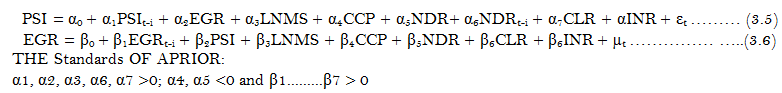
PSI = f (EGR, NMS, CCP, NDR, CLR, INR, PSIt-I)…………………………………………………………………………………….(3.3)

EGR = f (PSI, NMS, CCP, NDR, CLR, INR, EGRt-i )…………………………………………………… (3.4)

Model 3.4 and 3.5 econometric form is specified in an ARDL model format as dictated by the selection criterion for the model. That is captured respectively in Equations 5 and 6.

4. Analysis Data, and Results

The results of the regression from the above data and models are analysed here, and the results are discussed below.

Variables	@ Level	@ 1st Diff	@ 2nd Diff	Crit. Value	Order of Integration
NMS	-2.7830	-	-	-2.6388	I(0)
CC P	-5.7097	-	-	-3.5847	I(0)
CLR	-2.0982	-11.9718	-	-4.1658	I(1)
INR	-3.4157	-	-	-3.1830	I(0)
NDR	-0.7287	-6.5363	-	-4.1658	I(1)
EGR	-3.4629	-	-	-3.1883	I(0)
PSI	-4.4941	-	-	-4.1611	I(0)

Variables	@ Level	@ 1st Diff	@ 2nd Diff	Crit. Value	Order of Integration
NMS	-3.5272	-	-	-3.5107	I(0)
CC P	-2.4318	-6.1762	-	-4.1658	I(1)
CLR	-4.6400	-	-	-3.5064	I(0)
INR	-3.2928	-	-	-3.1830	I(0)
NDR	-0.7834	-6.5254	-	-4.1658	I(1)
EGR	-6.3641	-	-	-4.4868	I(0)
PSI	-4.4868	-	-	-4.1611	I(0)

Note: The check was with pattern and Intercept at 5 per cent LOS.

Tables 1 and Table 2 figures are stationarity test results. It shows that all variables were stationary at levels, except for CLR, CCP and NDR, which after the first difference became stationary. The result obtained in both ADF and PP tests has a mixture of stationary and non-stationary results. The result told my use of ARDL further.

4.1. Data Analysis

4.1.1. Selection Criteria Figure

4.1.1a. Selection Criteria for the Lagoons

From Figure 1a and Table 3b, the Information Criterion showed that the most suitable model for this analysis is ARDL (1,0,0, 1, 0, 0, 0.) It reiterated ARDL methodology that variables need not necessarily have the same lag(s) in the analysis, as opposed to that of VAR where all variables are given the same lag(s). The correct lag selection helps to avoid misspecification problem.

4.1.2. Estimated Long-Term Experiment

The model measured impact of the monetary instrument on private domestic investment in Nigeria: 1970-2018 using the ARDL model and the result is shown in Table 4.

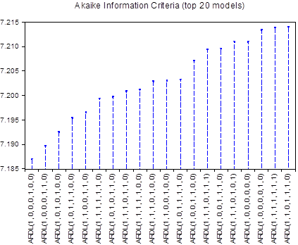
Figure-1a. Akaike model selection by figures.

AIC*	BIC	HQ	Adj. R-sq	Specification
7.186933	7.548266	7.321635	0.566405	ARDL(1, 0, 0, 0, 1, 0, 0)***
7.189664	7.591145	7.339332	0.572238	ARDL(1, 0, 0, 0, 1, 1, 0)
7.192487	7.593967	7.342155	0.571029	ARDL(1, 0, 1, 0, 1, 0, 0)
7.195347	7.636976	7.359982	0.576398	ARDL(1, 0, 1, 1, 1, 0, 0)
7.196514	7.638142	7.361149	0.575904	ARDL(1, 1, 0, 0, 1, 1, 0)
7.199332	7.721257	7.393900	0.586559	ARDL(1, 1, 1, 1, 1, 1, 0)
7.199651	7.641280	7.364286	0.574571	ARDL(1, 0, 1, 0, 1, 1, 0)
7.200813	7.682589	7.380414	0.580246	ARDL(1, 1, 1, 0, 1, 1, 0)
7.201170	7.682946	7.380771	0.580097	ARDL(1, 1, 1, 1, 1, 0, 0)
7.202838	7.644466	7.367472	0.573213	ARDL(1, 1, 1, 0, 1, 0, 0)

Note: * * * This means the ARDL model is chosen according to the selection criteria.

Estimated coefficients use of the ARDL (1,0,0,0,1,0,0) selected based on the criterion of Akaike data (AIC)
Dependent variable is PDI
Regressor	Coefficient	Std. Error	t-Statistic	Prob.*
PDI(-1)	0.281614	0.135191	2.083085	0.0440*
EGR	0.251796	0.302079	0.833542	0.4097
LNMS	-6.329004	1.788600	-3.538525	0.0011**
CCP	1.821768	0.587625	3.100221	0.0036**
NDR	-0.060677	0.084386	-0.719032	0.4765
NDR(-1)	0.127702	0.087740	1.455459	0.1538
CLR	0.096018	0.331891	0.289305	0.7739
INR	-0.053557	0.103084	-0.519554	0.6064
C	30.23677	8.864749	3.410900	0.0015**
R2                 = 0.605631       Adjusted R2 =   0.522606. S.E. of Regression    = 9.499019       F-statistic (Prob.)   =   7.294566 (0.000008)
Diagnostic Tests:
Test Statistics                                                          LM Version
A. Serial Correlation                            Х2 auto      = 2.349682 (0.1099) B. Functional Form (Ramsey Reset)   Х2 RESET      = 1.577798 (0.2170) C. Normality                                        Х2 Norm      = 32.85101 (0.000000) D. Heteroscedasticity                            Х2 Het       = 1.748645 (0.1186)

Note: * * and * signify importance at the sense stage of 1 per cent and 5 per cent. Figures are probability values in parenthesis. A is LM Test of Breusch-Godfrey serial correlation, B is RESET test of Ramsey, C is test of normality, D is test of heteroscedasticity.

The result shown in Table 4 indicates Nigeria's projected long-term monetary instrument effects model for private domestic investment: 1970-2018. Obviously, PDI(-1) and CCP have positive and important consequences on the dependent variable. LNMS retained a negative sign but the dependent variable had a significant impact. Also, to illustrate the goal variable, PDI, EGR, NDR, (NDR-1), CLR, and INR were not relevant at 5 percent LOS.

Given the results provided, a PDI(-1) unit change leads to a PDI change of 0.281614. A percent change in LNMS also contributes to a change in PDI of -6.329004.  A unit increase in private sector commercial bank credit (CCL) in its current period leads to an increase of 1.821768 in private domestic credit in Domestic Private Investment (PDI).
However, the determination coefficient (R2) showed that approximately 61% of variations in private domestic investment in Nigeria are explained by explanatory variables above 50%, and even after taking into account the degree of freedom, the modified R2 still showed that the explanatory variety explains 52% variation in private domestic investment. At 5 percent LOS, the F-statistic 7.294566 (0.00008) validated the fitness of the determination coefficient as important.

Also, diagnostic tests such as Breusch-Godfrey Serial Correlation, Ramsey's RESET test, Normality test and Heteroscedasticity test further affirm the validity of these findings.  The findings are shown in table 4.1.2 and it does display all the diagnostic tests passed by the sample. The diagnostic tests applied to the model show evidence that there is no serial association or heteroscedasticity. In addition, the RESET check asserts that the ARDL model was defined correctly. Residual skew and kurtosis based on normality testing showed that the residuals are normally distributed.

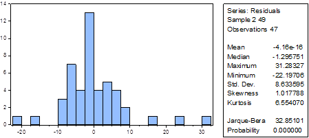
Figuer-2(A). The measure of normality.

Using the Cumulative Sum (CUSUM) and Cumulative Sum of Square (CUSUMSQ), the consistency of the regression coefficients is further evaluated. The CUSUM and CUSUMSQ plotting showed that the regression equation is found to be stable, provided that neither the CUSUM nor the CUSUMSQ test statistics go beyond the 5 percent significance level stipulated limits.

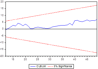
Figure-2(B). Stability (CUSUM) tests.

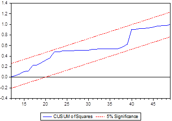
Figure-2(C). Stability tests.

4.1.3. ARDL Binding Test Approach to Cointegration

The binding test approach to cointegration attempts to validate whether there is a long-term relationship between the variables in the model. That was achieved by checking whether or not the coefficients in our estimated model are equal to zero. Table 5 shows the F-Statistic value from the bound check and its critical value;

Null Hypothesis: No long period relationships exist
Test Statistic	Value	K
F-statistic	4.334158	6
Critical Value Bounds
Significance	I(0)	I(1)
10%	1.99	2.94
5%	2.27	3.28
2.5%	2.55	3.61
1%	2.88	3.99

Test results for the ARDL bounds F are listed in Table 5.  The results confirm the existence in the model for the duration under consideration of a long-term relationship between private domestic investment in Nigeria (PDI) and the independent variables. That is because the F- figures measured at 4.334158 is higher than the upper critical values at 1%, 5% and 10% meaning levels. Inferring, therefore, that a co-integrating relationship exists between the time series in the level form, without considering whether they are I(0) or I(1). In other words, the non-co-integration hypothesis may be rejected at the level of 1%, 5% and 10%, since the F test statistics are higher than the critical upper limit value I(1).

4.1.4. Short-Term Description of ARDL Dynamics and Error Correction

After verifying the existence of a long-term relationship between variables, it is necessary to estimate both of the model's error correction mechanism along with its long-term shape. First used by Sargan (1964) and popularized by Granger and Engel (1987) the model for correction of errors.

The diagnostic tests also tested the model for the unregulated correction of errors (bounds test). These included Lagrange multiplier test of residual serial correlation, Ramsey's RESET test, Jarque-Bera test of normality, based on residual skewness and kurtosis measurements, and Breusch-Godfrey test of heteroscedasticity, based on square residual regression on the initial model regressors.

Dependent variable is PDI
Regressor	Coefficient	Std. Error	t-Statistic	Prob.*
D(NDR)	-0.060677	0.064731	-0.937368	0.3545
CointEq(-1)*	-0.718386	0.112110	-6.407842	0.0000**

Note:** and* indicate meaning at 1 per cent and meaning level at 5 per cent. Figures are probability values in parenthesis. A is LM Test of Breusch-Godfrey Serial Correlation, B is RESET test of Ramsey, C is test of normality, D is test of heteroscedasticity.

The result in Table 6 implies that all variables are at level except for PDI and NDR that have a 0 (zero) lag from the chosen model: ARDL (1,0,0,0,1,0,0), this means that the PDI and NDR effects are not instantaneous. The effects of all other independent variables on the target variable are instantaneous though the lag of dependent variable is influencing the complex responses. In other words, its contemporary values govern the complex response of dependent variable to the shock of these variables. Hence, the short time parameter in the initial ARDL result is identical to the instantaneous parameter. In addition, the magnitude of the calculated error correction coefficient suggests a relatively high level of adjustment to any disequilibrium. In other words, the average ECM (-1) (Coint Eq(-1)*) is equivalent to -0.718386 which means that the equilibrium departure is changed by approximately 72 percent per year. This is also negative, important and less than one which means that you will rely on information from this for policy decisions.

4.1.5. Lag Selection Criteria

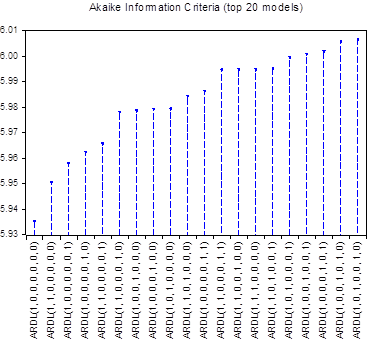
Figure-3. Lag selection criteria.

AIC*	BIC	HQ	Adj. R-sq	Specification
5.935117	6.256302	6.054851	0.097389	ARDL(1, 0, 0, 0, 0, 0, 0)
5.950456	6.311789	6.085157	0.098928	ARDL(1, 1, 0, 0, 0, 0, 0)
5.957900	6.319232	6.092601	0.092196	ARDL(1, 0, 0, 0, 0, 0, 1)
5.962400	6.323733	6.097101	0.088101	ARDL(1, 0, 0, 0, 0, 1, 0)
5.965720	6.367200	6.115388	0.099838	ARDL(1, 1, 0, 0, 0, 0, 1)
5.978113	6.379593	6.127781	0.088613	ARDL(1, 1, 0, 0, 0, 1, 0)
5.978646	6.339978	6.113347	0.073166	ARDL(1, 0, 0, 1, 0, 0, 0)
5.979301	6.340634	6.114002	0.072558	ARDL(1, 0, 0, 0, 1, 0, 0)
5.979412	6.340744	6.114113	0.072456	ARDL(1, 0, 1, 0, 0, 0, 0)
5.984360	6.385841	6.134028	0.082901	ARDL(1, 1, 0, 1, 0, 0, 0)

Note:* This means the ARDL model is selected according to the selection criteria.

The knowledge criterion given in Figure 3 and Table 7 showed that the model is suited to the ARDL (1, 0, 0, 0, 0, 0, 0.). This illustrates the benefit of ARDL methodology since it is not mandatory for all variables to have the same lag(s) in comparison to VAR in which all variables are given the same lag(s). The optimum selection of lags should be considered as this may result if overlooked, in the question of misspecification and autocorrelation.

4.1.6. Estimated Long-Term Model

The second model for determining the impact of private domestic investment and monetary instruments on Nigeria's economic growth: 1970-2018 was estimated using the ARDL model and the findings are described in Table 8.

The outcome presented in Table 8 indicates that the approximate long duration of the second iteration of an assessment of the impact of private domestic investment and monetary instruments on Nigerian economic growth: 1970-2018. EGR (-1) was not important in the interpretation of the dependent variable as a result. At 10 percent, PDI was significant. In addition, both LNMS and NDR are important in explaining the dependent variable at 5 percent LOS; while CCP, CLR and INR were negligible in evaluating economic growth in Nigeria during the study period.

Estimated Long Period Coefficients Using the ARDL (1,0,0,0,0,0,0) Selected based on Akaike info criterion (AIC)
Dependent variable is EGR
Regressor	Coefficient	Std. Error	t-Statistic	Prob.*
EGR(-1)	-0.072433	0.155163	-0.466818	0.6433
PDI	0.120173	0.069348	1.732899	0.0912*
LNMS	1.886111	0.894890	2.107646	0.0417**
CCP	-0.015983	0.284713	-0.056138	0.9555
NDR	-0.048893	0.019279	-2.536089	0.0154**
CLR	0.146564	0.146275	1.001976	0.3227
INR	-0.056965	0.046192	-1.233236	0.2251
C	-8.218182	4.475459	-1.836277	0.0741*
R Squared                 = 0.726887       Adjusted R-Squared =   0.704471                     S.E. of Regression    = 4.330436       F-statistic (Prob.)   = 1.593131 (0.000014)
Diagnostic Tests:
Test Statistics                                                          LM Version
A. Serial Correlation                            Х2 auto      = 0.018022 (0.9821) B. Functional Form (Ramsey Reset)   Х2 RESET      = 2.766368 (0.1047) C. Normality                                        Х2 Norm      = 32.85101 (0.000000) D. Heteroscedasticity                            Х2 Het       = 2.946435 (0.4144)

Note: * * and * indicate meaning at 1 per cent and meaning level at 5 per cent. Figures are probability values in parenthesis. A is LM Test of Breusch-Godfrey Serial Correlation, B is RESET test of Ramsey, C is test of normality, D is test of heteroscedasticity.

The result shows that an increase in PDI unit leads to an increase in Nigeria's economic growth rate of 0.120173. A percentage increase in LNMS brings in a boost in economic growth rate of 1. 886111. A shift of unit in NDR results in a change of the goal variable (EGR) to -0.0048893. PSI and NMS therefore positively impact economic growth rate among the significant independent variables; while NDR exerts negative influence on the EGR for the period under consideration. The determination coefficient (R2) shows that the explanatory variables above 50 per cent explain approximately 73 percent of variations in the economic growth rate and even after taking into account the degree of freedom, the modified R2 only shows that the explanatory variables explain 70 per cent variance in economic growth. In describing the dependent variable, the F-statistic 1.593131 (0.000014) confirmed the fitness of the determination coefficient and indicates an overall significant level of the explanatory variables jointly.

A few diagnostic tests such as Breusch-Godfrey Serial Correlation LM Test, Ramsey's RESET test, Normality Test, and Heteroscedasticity test were used to further test the outcome. The outcome of these tests as shown in Table 8 indicates that all diagnostic tests were passed by the device. The diagnostic tests applied to the model show that there is no proof of serial correlation and heteroscedasticity because their likelihood values are all above 5%. In addition, the RESET test means that the ARDL model was correctly defined and that the residuals were distorted and kurtosis residuals dependent on the normality test show normal distribution of the residuals.

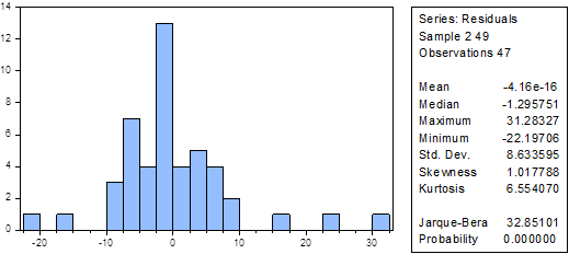
Figure-4(a). Normality test.

The stability of the regression coefficients was evaluated using the cumulative sum (CUSUM) and the cumulative square sum (CUSUMSQ) of the residual structural stability test recursively. CUSUM and CUSUMSQ plots demonstrate that the regression equation tends to be stable provided that neither the CUSUM nor the CUSUMSQ test statistics go beyond the value point of 5 per cent.

Figure-4(b). Stability (CUSUM) tests.

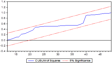
Figure-4(C). Stability (CUSUM) tests.

4.1.7. ARDL Bound Test Approach to Cointegration

The cointegration bound test method aims to validate whether there is a long-term relationship between the variables in the model. This is achieved by checking whether or not the coefficients in our calculated model are equal to null. Table 9 presents the F-Statistic value from the bound test and the critical value boundary as shown by the result provided by E-views 10.

Null Hypothesis: No long period relationship exist
Test Statistic	Value	K
F-statistic	6.257098	6
Critical Value Bounds:
Significance	I(0)	I(1)
10%	1.99	2.94
5%	2.27	3.28
2.5%	2.55	3.61
1%	2.88	3.99

ARDL bounds F test results as stated in Table 9 shows that the result confirms the existence in the model for the duration under consideration in Nigeria of a long-term relationship between economic growth rate (EGR) and independent variables. This is because the F figures measured are 6,257098 and is higher than the upper critical values at 1%, 5% and 10% significance rates. And thus, inferring that a co-integrating relationship exists between the time series in the level form, without considering whether they are I(0) or I(1). In other words, the non-co-integration hypothesis can be dismissed at the sense level of 1%, 5% and 10%, since the F test statistics are higher than the critical upper limit value I(1).

4.1.8. Short Duration Dynamics and Error Correction Representation of ARDL Cointegrating

Once the presence of a long-term relationship between the variables is established, it is important to estimate both the model's error correction mechanism and its long-term shape. The diagnostic tests from the unregulated error correction (bounds test) model were also analysed. These include the Lagrange multiplier test of residual serial correlation, the RESET test by Ramsey using the square of the fitted values for proper functional form (no mis-specification), the Jarque-Bera normality test based on residual skew and kurtosis measurements and the heteroscedastic Breusch-Godfrey.

Dependent variable is EGR
Regressor	Coefficient	Std. Error	t-Statistic	Prob.*
CointEq(-1)*	-0.672433	0.087338	-7.699206	0.0000***

Note: *** and * indicate significance at 1% and 5% level of significances. Figures in parenthesis are probability values. A is Breusch-Godfrey Serial Correlation LM Test, B is Ramsey’s RESET test, C is Normality Test, D is Heteroscedasticity test.

The finding presented in Table 10 indicates that the EGR effects are not instantaneous, although not significant, while the effects of all other independent variables on the target variable are instantaneous. It does mean, however, that the dynamic responses are influenced by the lag of dependent variable. In other words, its contemporary values govern the complex response of dependent variable to the shock of these variables. Hence, the short duration parameter in the initial ARDL result is similar to the instantaneous parameter. In addition, the magnitude of the calculated error correction coefficient term indicates a relatively high level of adjustment to any short-term disequilibrium. In other words, the Coint Eq (-1) estimate is equivalent to -0.672433 which states that the departure from the equilibrium is modified by around 67 percent per year. It is also negative, important and that means that you can rely on information from this for policy decisions.

5. Resumé and Conclusion

The research outcome is relatively revealing. The tests verified the obvious variables that affected the dependent variable, PDI, significantly. The one-period PDI and Commercial Bank Credit to Private Investors (CCP) showed a positive and significant impact at 5 percent level. It means that the previous year's private domestic investment and commercial banks volume of credit were what positively drove private domestic investment in Nigeria over the study period. The narrow money supply (NMS) also had a negative but significant impact on domestic private investment. This result shows that most of the narrow supply of money goes to the economy's public sector.  It is also worth noting that monetary policy variables such as the Naira Dollar Rate (NDR), Commercial Bank Lending Rate (CLR) and Economic Growth Rate (EGR) did not have any significant impact on Nigeria's private domestic investment. These findings are in line with Onuorah and Chigbu (2012); Hassan (2015) and Ajayi and Kolapo (2018). Their results differently suggest that monetary instruments have a significant effect on Nigeria's private domestic investment; GDP growth rate has no significant impact on private domestic investment. Once again, the commercial bank credit affects private domestic investment substantially and positively. These studies also indicate that private domestic investment is more sensitive to the supply of money, and less sensitive to inflation and interest rates.From the second model, the findings show that private domestic investment (PDI) (although at 10 per cent LOS), narrow money supply (NMS) and naira-dollar exchange rate (NDR) explained economic growth rate (EGR) significantly. The majority of the explanatory variables, including the one-period lag in economic growth rate (EGR), were not significant to explain the model.

References

Adeolu, O. O. (2017). Foreign capital flows and economic growth in selected Sub-Saharan African econ omies. PhD Dissertation, Stellenbosch University. 

Adigwe, P., Echekoba, F., & Onyeagba, J. B. (2015). Monetary policy and economic growth in Nigeria: A critical evaluation. IOSR Journal of Business and Management, 17(2), 110-119.

Ajayi, L. B., & Kolapo, F. T. (2018). Is domestic private investment sensitive to macroeconomic indicators? Further evidence from Nigeria. World Journal of Economics and Finance, 4(2), 100-105.

Alexander, E. W. (1995). The adoption of indirect instruments of monetary policy. Paper presented at the Delivered During the course on Exchange Rate Management and the Conduct of Monetary Policy Organized by the West African Institute for Financial and Economic Management (WAIFEM), Lagos, Nigeria.

Alley, I. (2017). Capital flow surges and economic growth in Sub-Saharan Africa: Any role for capital controls? Working Paper Series, No 252. African Development Bank, Abidjan, Coted'Ivoire.

Bosco, A. S., & Emerence, U. (2016). Effects of gross domestic product, interest rate and inflation on private investment in Rwanda. International Academic Institute for Science and Technology, 3(1), 001-017.

CBN. (1992). The evolution and performance of monetary policy in Nigeria in the 1980's. CBN Bullion.

Chipote, P., & Makhetha-Kosi, P. (2014). Impact of monetary policy on economic growth: A case study of South Africa. Mediterranean Journal of Social Sciences, 5(15), 76-84.

Chuku, A. C. (2009). Measuring the effect of monetary policy innovations in Nigeria: A structural vector autoregressive approach. Africa Journal of Accounting, Economics and Banking Research, 5(5), 112-129.

Combey, A. (2016). The main determinants of private investment in the WAEMU zone: The dynamic approach. Munich Personal RePEc Archive Papers No 8.

Diabate, N. (2016). An analysis of long run determinants of domestic private investment in Cote d’Ivoire. European Scientific Journal, 12(28), 240-251.Available at: https://doi.org/10.19044/esj.2016.v12n28p240 .

Ekpo, U. N. (2014). The nexus of macroeconomic policy, investment and economic growth in Nigeria. Journal of Economics and Finance, India, 3(4), 12-22.Available at: https://doi.org/10.9790/5933-0341222 .

Ekpo., U. N. (2016). Determinants of private investment in Nigeria: An empirical exploration. Journal of Economics and Sustainable Development, 7(1), 080-092.

George-Anokwuru, C. C. (2017). Interest rate and private domestic investment in Nigeria. International Journal Economics and Business Management, 3(5), 043-049.

Gimba, V. K. (2015). An evaluation of the impact of monetary policy on the real sector in Nigeria. Mediterranean Journal of Social Sciences, 6(2), 361.Available at: 10.5901/mjss.2015.

Giwa, R. F. (1996). The role of the public and the private sector in economic development. CBN Economic and Financial Review, 3(4), 891-902.

Granger, C. W. J., & Engel, R. F. (1987). Co-integration and error correction: Representation, estimation, and testing. Econometrica, 2(2), 51-76.

Gujarati, D. N. (2009). Basic econometrics. New York, Boston: McGraw-Hill Inc.

Hassan, O. M. (2015). The impact of monetary policy on private capital formation in Nigeria. Journal of Empirical Economics, 4(3), 138-153.

Ihugba, O. A., Ebomuche, N. C., & Ezeonye, R. C. (2015). Relationship between economic growth and inflation in Nigeria:1970 - 2013. International Journal of Research in Business Studies and Management, 2(7), 14-22.

Irefin, D., & Yaaba, B. N. (2017). Determinants of foreign reserves in Nigeria: An autoregressive distributed lag approach. CBN Journal of Applied Statistics, 2(2), 63-75.

Johansen, S., & Juselius, K. (1990). Maximum likelihood estimation and inference on cointegration—with applications to the demand for money. Oxford Bulletin of Economics and statistics, 52(2), 169-210.Available at: https://doi.org/10.1111/j.1468-0084.1990.mp52002003.x .

Johansen., S. (1988). Co-integration and error correction: Representation. Estimation, and Testing, Econometrics, 4, 87-99.

Liang, Q., & Cao, H. (2005). The impact of monetary policy on property prices: Evidence from China. Tianjin, China. 300071: Nankai University,.

Mehdi, S., & Reza, M. (2011). Effects of monetary policy on industry sector growth in Iran. European Journal of Experimental Biology, 1(4), 29-40.

Ndikumana, L. (2016). Implications of monetary policy for credit and investment in Sub-Saharan African countries. Journal of African Development, 18(2), 1-18.
Nemedia, C. (2006). Elements of macroeconomic management: Monetary policy. Paper presented at the Regional Programme on Macro-econometric Modeling and Policy Analysis, organized by the West African Institute for Financial and Economic Management (WAIFEM), Lagos, Nigeria.

Nnanna, O. J. (2004). Finance, investment and growth in Nigeria (pp. 111). Garki, Abuja: A Central Bank of Nigeria Publication.

Nuhu, M. (2019). Effect of foreign private capital on economic growth in Nigeria: 1986-2017. The Nigerian Journal of Economics and Social Studies, 61(2), 211-229.

Nwakoby, C. I. N., & Alajekwu, U. B. (2016). Effect of monetary policy on Nigerian stock market performance. International Journal of Scientific Research and Management, 4(9), 4530-4442.

Nwoko, N. M., Ihemeje, J., & Anumadu, E. (2016). The impact of monetary policy on the economic growth of Nigeria. African Research Review, 10(3), 192-206.

Ogboru, l. (2010). Macroeconomics. Kaduna: Liberty Publications.

Ojo, M. O. (1998). The objectives, design and implementation of monetary Policy. Paper presented at the Delivered During the Course on Exchange Rate Management and the Conduct of Monetary Policy, Organized by the West African Institute for Financial and Economic Management (WAIFEM), Lagos, Nigeria.

Okezie, A. I. (2015). Effect of Nigeria expansionary monetary policy on investment growth. Paper presented at the 33rd The IIER International Conference, Berlin, Germany, 26th August 2015.

Okoro, A. (2013). Impact of monetary policy on Nigerian economic growth. Prime Journal of Social Science, 2(2), 195-199.

Okoroafor, D. O., Adeniji, S. O., & Olasehinde, T. (2018). Estimating and forecasting the impact of inflation on economic growth in Nigeria using threshold analysis. CBN Journal of Applied Statistics, 9(1), 1-22.

Olanrewaju, H. M. (2015). The impact of monetary policy on private capital formation in Nigeria. Journal of Empirical Economics, 4(3), 138-153.

Onuorah, A. C., & Chigbu, E. E. (2012). Long run relationship between private investment monetary policy in Nigeria. Journal of Business and Management Review, 1(10), 45-55.

Onuorah., C. O., Omade, I. S., Edwin, O., & Izien, O. F. (2011). The impact of monetary policy on micro-economic and private investment in Nigeria. Research Journal of Finance & According, 2(3), 66-75.

Osemeke, M. (2011). Problems and prospects of private sector organisations in Nigeria. International Journal of Business and Management, 6(4), 178 -187.

Pesaran, M. H., Shin, Y., & Smith, R. J. (2001). Bounds testing approaches to the analysis of level relationships. Journal of Applied Econometrics, 16(3), 289-326.Available at: https://doi.org/10.1002/jae.616 .

Sargan, J. D. (1964). Wages and prices in the United Kingdom: A study in econometric methodology. Econometric Analysis for National Economic Planning, 16, 25-54.

Sesay, B., & Brima, A. S. (2017). Monetary policy effect on private sector investment: Evidence from Sierra Leone. International Journal of Economics and Financial Issues, 7(1), 476-488.

Tobias, O., & Mambo, C. (2012). The effect of monetary policy on private sector investment in Kenya. Journal of Applied Finance & Banking, 2(2), 1-9.

Appendix

Monetary and Some Other Macroeconomics Variables
YEAR	NMS	CCP	CLR	INR	NDR	EGR	PDI
1970	9.81	3.86	8	13.8	0.7143	-	28
1971	10.41	4.8	10	10	0.6955	18.2	32
1972	12.05	5.45	10	3.2	0.6579	7.7	31
1973	15.08	5.96	10	6.4	0.6579	2	65.1
1974	27.3	4.62	10	13.4	0.6299	12	41.3
1975	41.79	6.43	9	33.9	0.6159	-3	27.7
1976	58.45	7.21	10	21.2	0.6265	10.9	22.6
1977	78.14	8.74	6	15.4	0.6466	8.2	34.9
1978	75.2	10.71	11	16.6	0.606	-7.4	39.2
1979	98.49	10.16	11	11.8	0.5957	2.6	36.2
1980	14.39	12.03	9.5	9.9	0.5464	5.3	30.8
1981	14.47	5.73	10	20.9	0.61	-8.5	28
1982	15.79	6.38	11.75	7.7	0.6729	-0.3	30.7
1983	17.69	6.15	11.5	23.2	0.7241	-5.4	28.9
1984	20.11	6.21	13.5	39.6	0.7648	-5.1	24.1
1995	22.30	5.99	11.75	5.5	0.8938	9.3	22.3
1986	23.81	7.53	12	5.4	2.0206	2.6	28.6
1987	27.57	6.56	19.2	10.2	4.0179	9.9	29.9
1988	38.36	6.01	17.6	38.3	4.5367	7.4	31
1989	45.90	5.04	24.6	40.9	7.3916	8.2	41.9
1990	47.42	4.95	27.7	7.5	8.0378	4.7	36.7
1991	75.40	4.99	20.8	13	9.9095	3	17
1992	111.11	8.17	31.2	44.5	17.2984	2.7	16
1993	165.34	6.94	18.32	57.2	22.0511	1.3	14.6
1994	230.29	7.99	21	57	21.8861	2.2	15
1995	289.09	6.49	20.79	72.8	21.8861	3.3	11
1996	345.85	6.15	20.86	29.3	21.8861	3.4	9
1997	413.28	7.01	23.32	8.5	21.8861	3.2	9.5
1998	488.15	7.61	21.34	10	21.886	2.5	9
1999	628.95	8.15	27.19	6.6	92.5284	2.8	7
2000	878.46	8.22	21.55	6.9	109.5500	3.8	6.5
2001	1,269.32	9.84	21.34	18.9	113.4500	1.4	8
2002	1,505.96	8.07	30.19	12.9	126.9000	3.4	9
2003	1,952.92	8.9	22.88	14	137.0000	2.3	9.7
2004	2,131.82	8.45	20.82	15	132.8500	3.4	10.6
2005	2,637.91	8.43	19.49	17.9	129.0000	2.6	7.4
2006	3,797.91	8.11	18.70	8.22	127.0000	2.7	8.7
2007	5,127.40	14.84	18.36	5.4	116.8000	7.3	25
2008	8,008.20	20.78	18.70	11.58	131.2500	7.2	5.99
2009	9,411.11	22.27	22.62	12.54	148.1000	8.4	48.59
2010	11,034.94	15.63	22.51	13.74	148.8127	11.3	31.58
2011	12,172.49	12.58	22.42	10.83	156.7000	4.9	7.78
2012	13,893.22	11.83	23.79	12.23	157.2500	4.3	3.89
2013	15,154.64	12.59	24.69	8.5	159.9000	5.4	11.63
2014	16,238.52	14.49	25.74	8	180.0000	6.3	18.45
2015	18,525.22	14.19	26.71	9	197.0000	2.7	3.8
2016	21,624.63	15.66	27.29	15.7	305	-1.6	6.84
2017	22,363.43	14.16	30.68	16.5	306	0.8	12.15
2018	25,079.72	10.91	31.09	12.09	307	1.9	19.8

Source: Central Bank of Nigeria Statistical Bulletin, (various issues) and World Economic Indicators.