Capital Asset Pricing Model (CAPM) Study in Mean-Gini Model 

 

Jamal Agouram^1*
Jamaa Anoualigh²
Ghizlane Lakhnati³

1,2Faculty of Law, Economics and Social Sciences, Ibn Zohr University of Agadir, Morocco. 3National School of Applied Sciences (ENSA), Agadir, Morocco.	Abstract The valuation of financial assets is taking on an important dimension today. It is at the heart of turbulent financial actuality as it helps in understanding and quantifying the relationship between the risk and the return on financial assets. Traditionally, the Capital Asset Pricing Model (CAPM), developed by Sharpe (1964);Lintner (1965) and Mossin (1966) has been essential for understanding this relationship. This model is unquestionably the most well-known valuation model used since its empirical validation by several studies (Black, Jensen, and Scholes (1972); Fama and James (1973)). Unfortunately, several empirical studies have weakened this model by showing the existence of various anomalies (Bantz (1981); Chan and Chen (1991); Basu (1977); Fama and French (1992); Fama and French (1993)). Later, Shalit and Yitzhaki (1984) developed an alternative based on the Mean-Gini model while retaining the main assumptions of the classic CAPM. However, instead of holding efficient medium-variance portfolios, investors build market portfolios that are effective Mean-Gini subsets. This article presents and compares the financial asset valuation models: CAPM derived from Mean-Variance and CAPM derived from Mean-Gini. The results show that the two models are very close in terms of valuation of asset returns.
Licensed: This work is licensed under a Creative Commons Attribution 4.0 License.
Keywords: Arbitrage pricing theory Capital market line CAPM Gini coefficient Mean-Gini Mean-Variance Risk. JEL Classification G10; O16.
Accepted: 19 May 2020 Published: 8 June 2020
(* Corresponding Author)

Funding: This study received no specific financial support.

Competing Interests:  The authors declare that they have no competing interests.

1. Introduction

Markowitz (1952); Markowitz (1952b); Markowitz (1959) Mean-Variance model is not sufficient for portfolio optimization, unless the returns follow a normal distribution. This model remains an essential reference in portfolio management given its historical importance as a benchmark model. But, this approach has been criticized and has given rise to several other models (Mean-Gini, Mean-Semi Variance, Mean-absolute deviation, Mean-VaR). A few years later and on the basis of the work of Markowitz, Sharpe (1964); Lintner (1965) and Mossin (1966) developed the Capital Asset Pricing Model (CAPM), which leads, according to certain hypotheses, to the equilibrium relationship between the expected return on any financial asset and its risk. The Capital Asset Pricing Model (CAPM) aims to resolve the problem of the relationship between asset prices and the various components of total risk. It provides an efficient way to analyze the factors that affect asset prices using a linear regression model.

Then, in the late 1970s, Ross (1976) developed an alternative multifactorial model to the CAPM called Arbitrage Pricing Theory (APT). This model assumes that in a fully competitive market, arbitrage opportunities do not exist. Unlike CAPM, this maintains that the return on financial assets is the result of the integrated effects of various factors (such as GDP growth, inflation rate, etc.) and isn’t only affected by risk factors internal to the portfolio. Markowitz's model, CAPM and APT thus constitute the core of classic portfolio theory. In this same framework, an extension of CAPM and APT, the model of Fama and French (1992); Fama and French (1993) was born to compensate the contradictory evidence shown in several empirical studies (Basu (1977); Hansen and Singleton (1982); Bhandari (1988); Jegadeesh (1990); Campbell and Cochrane (2000) and Parker and Julliard (2005)). It is a three-factor model which offers an original specification since it explains the return as a function of a systematic risk factor and two specific risk factors. Subsequently, Fama and French (2015) extended the three-factor model to a five-factor model to explain the returns of their sample and the results showed the superiority of the five-factor model. These models have been the subject of several studies to test their power on international data (Fama and French (2016);  Yaşar (2017); Belimam and Lakhnati (2018) and Belimam, Tan, and Lakhnati (2018)).

Yitzhaki (1982) originally developed The Mean-Gini (MG) model and then it was applied to finance by Shalit and Yitzhaki (1984) as an alternative model to the Mean-Variance model. Agouram and Lakhnati (2015a); Agouram and Lakhnati (2015b) show that the Mean-Gini (MG) model presents solid results when the Mean-Variance model isn't appropriate, especially when assets are not normally distributed. The Mean-Gini (MG) model is like the Mean-Variance model because it also uses two summary statistics: Mean and the Gini coefficient.

In the optimal choice process of the portfolio, the Gini coefficient is preferable to the variance, because the Mean-Gini (MG) model encompasses both propositions asserting the necessary and sufficient conditions for second-degree stochastic dominance (SSD), as pointed out by Yitzhaki (1982). Besides, the Mean-Gini model has also been extended to take into account the risk aversion (Yitzhaki (1983) and Agouram and Lakhnati (2016)).  The Mean-Extended Gini Model (MEG) allows the introduction of specific risk aversion in portfolio selection. Shalit and Yitzhaki (1984) keep the main assumptions of classical CAPM. But, instead of holding efficient Mean-Variance portfolios, investors build market portfolios that are subsets of effective Mean-Gini.

The purpose of this article is to present and compare the models of valuation of financial assets: Capital Asset Pricing Model (CAPM) derived from Mean-Variance and Capital Asset Pricing Model (CAPM) derived from Mean-Gini. 

2. Literature Review

2.1. The Capital Asset Pricing Model (CAPM)

The Capital Asset Pricing Model (CAPM) is a financial asset valuation model developed simultaneously by Sharpe (1964) and Lintner (1965) based on the work of Markowitz (1952) and Tobin (1958) on portfolio theory in a Mean-Variance context. This model, which has marked the development of modern finance, is one of the most important models of the modern theory of financial markets. Also, it is a reference for portfolio management.

This model is an extension of Markowitz's analysis, so some of the assumptions of this model are common to the Markowitz model. Sharpe developed the Capital Asset Pricing Model (CAPM), under three added assumptions: (a) financial markets are perfect in the sense that agents can lend and borrow in the absence of any quantitative constraint, (b) financial markets are perfectly competitive and (c) agents have the same expectations about returns. The latter implies that the efficient frontier is the same for all investors. Thus, all investors hold the same portfolio of risky assets and differ only in the weight x devoted to the risky asset and  for the risk-free asset. The weight x given to the risky asset is all the greater as the risk aversion of the investor concerned is low. The CAPM assesses the relevant risk of any financial asset (individual security or efficient portfolio) and establishes a relationship between the risk and the expected return on that asset.

Think about a rational investor who divides their wealth between risky assets and risk-free assets. Let  denote the return on risk-free asset, R denote that of an investment in a portfolio of risky assets and x be the proportion of total wealth invested in risky assets. Let P denote the resulting portfolio and  its random return.

We have the return on a portfolio P that can be written as Equation 1:

Equation 1 shows that the investor can maximize his expected return by an appropriate choice of x, but Equation 2 proves an increase in risk proportional to the number of risky assets included in the portfolio. Taking into account Equation 1 and Equation 2 we can deduce the value of x as in Equation 4.

The problem becomes an asset allocation problem and the investor has to divide his wealth between risky assets and riskless assets. The rational investor seeks to maximize return for a given level of risk or, conversely, to minimize risk for a given level of return. Nevertheless, the efficient frontier is the same for all agents. So, all investors, whatever their initial wealth and risk preferences, build their optimal portfolios by a combination of risk-free assets and the market portfolio. We now know that the market portfolio is in tangency with the Capital Market Line (CML). Mathematically, this implies that the curves of the CML and the efficient frontier at the market portfolio point are identical:

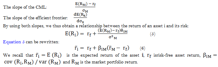
 Equation 6 expresses the fundamental relationship of the CAPM. It is valid for both a portfolio and an individual asset.

According to the CAPM principle, efficient portfolios are constructed by holding a combination of the market portfolio and the risk-free asset, the proportions being determined according to each investor's risk aversion.

2.2. The Capital Asset Pricing Model (CAPM) & Mean-Gini Model

Shalit and Yitzhaki (1984) retain the main assumptions of classical CAPM. However, instead of holding efficient mid-variance portfolios, investors build market portfolios that are subsets of effective Mean-Gini. To justify this approach, we put forward two avenues of consideration to infer investor behavior in the asset market: The first assumes that investors have a specific utility function that weighs the mean against the measure of dispersion represented by the Gini coefficient. Investors are allowed to borrow and lend at risk free rate, . The rate of return of the investor's portfolio is given by Equation 7:

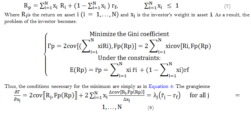
Based on the homogeneity property and Euler's theorem, Shalit and Yitzhaki (1984) obtained the relation between portfolio risk (the Gini coefficient) and its expected return as in Equation 9.

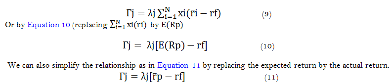
Shalit and Yitzhaki (1984) claim that the homogeneity of perception risk leads investors to hold identical portfolios of risky assets. In addition, in the theory of classical financial markets, for investors who hold the market portfolio, the price of risk will be

Shalit and Yitzhaki (1984) claimed that  Equation 15 represents the degree of responsiveness of the rate of return of security  as to changes in the market, and  is the proportion of total risk (expressed by the Gini coefficients of security) that cannot be/eliminated by the market without reducing the expected rate of return.

According to Shalit and Yitzhaki (1984) betas derived from classical CAPM and Mean-Gini coincide for the same observations but only when the perspectives are normally distributed. However, this is not always true for prospects that are not normally distributed. In general, the MV and MG betas will be different, the beta MGs corresponding to the efficient securities markets according to stochastic dominance.

3. Data and Methodology

The sample in our study consists of CAC40¹ stocks. Despite the existence of several stocks in the composition of this index, we restricted our field of study to five assets. The shares (the most active during this period) are Société Générale (GLE.PA), Veolia Environnement (VIE.PA), Air Liquide (AI.PA), Credit Agricole (ACA.PA), Accor (AC. PA).
The use of the data is as follows:

1. First, we use the first 1342 daily returns, corresponding to the period from September 29, 2010 to December 30, 2015, for estimating inputs for both CAPM models: Capital Asset Pricing Model (CAPM) derived from Mean-Variance and Capital Asset Pricing Model (CAPM) derived from Mean-Gini.
2. Secondly, we estimate the daily return of each asset for the period from January 4, 2016 to September 27, 2019.
3. Finally, the estimated returns and the actual returns observed will be compared through a back-testing procedure.

4. Empirical Results and Discussion

This empirical study begins with an analysis of the characteristics of the selected stocks. We define the tests and the coefficients that allow the detection of the normality of the series, and then we conduct our investigation on the distribution of the series studied.

(a) Study of the Normality of Returns: For a long time, the behavior of the return series of financial securities was considered normal. However, in reality, several empirical studies have shown that these series are non-normal. Their distributions are asymmetrical and display a leptokurtosis; they are often thicker at the ends and reveal thick tails.

Stocks	AC_PA	ACA_PA	AI_PA	CAC40	GLE_PA	VIE_PA
Mean	0.000412	0.000266	0.000330	0.000250	7.92E-05	0.000237
Median	0.000000	0.000000	0.000456	0.000431	-0.000119	0.000755
Maximum	0.093671	0.219622	0.052724	0.062784	0.225420	0.148612
Minimum	-0.094927	-0.140047	-0.084626	-0.080425	-0.205736	-0.188811
Std. Dev.	0.017891	0.023638	0.012492	0.011883	0.025218	0.018324
Skewness	-0.129321	0.332892	-0.220605	-0.213952	0.101237	-0.415468
Kurtosis	6.526587	9.974820	5.731501	6.420263	11.77179	12.75555
Jarque-Bera	1197.751	4702.545	733.3587	1138.130	7374.551	9182.713
Probability	0.00	0.00	0.00	0.00	0.00	0.00
Sum	0.946438	0.611697	0.758520	0.574260	0.182013	0.544928
Sum Sq. Dev.	0.735595	1.284015	0.358593	0.324497	1.461365	0.771629
Observations	2299	2299	2299	2299	2299	2299

The normality of the returns is checked from the econometric tests, which are based on the determination of the symmetry coefficients (Skewness) and flattening (Kurtosis). One of these tests is the Jarque-Bera test that synthesizes the two coefficients. The Jarque-Bera test is based on the Skewness coefficients and Kurtosis. It evaluates the simultaneous deviations of these coefficients with the reference values ​​of the normal distribution.

(b) Empirical results: Using the Jarque-Bera test on normality, we found that the distribution of the returns of the stocks does not follow a normal distribution and thus is at the threshold of a = 1%. The values ​​of the Jarque-Bera statistics for each stock are given in Table 1. They all exceed the critical value of the test, which is 9.83 for the threshold of a = 1%. The results in Table 1 show that the skewness coefficient is negative for some stocks and positive for others, which means that the left side of their distributions is thick (negative direction) and the opposite for those with positive coefficients, thus proving the asymmetrical behavior of the series of stocks studied. Also, the Kurtosis coefficient results are greater than 3, which means that the tails are thicker than that of the normal law (leptokurtic distribution). Consequently, the results of the normality test (Jarque-Bera) for each stock led us to reject the null hypothesis of the normality test at a 99% confidence level. These results have highlighted the well-known property of financial data series, namely  returns are not normally distributed. Besides, the properties of asymmetry and leptokurtic distribution have been discovered and are true for our data. Figure 1 illustrates the stocks’ returns.

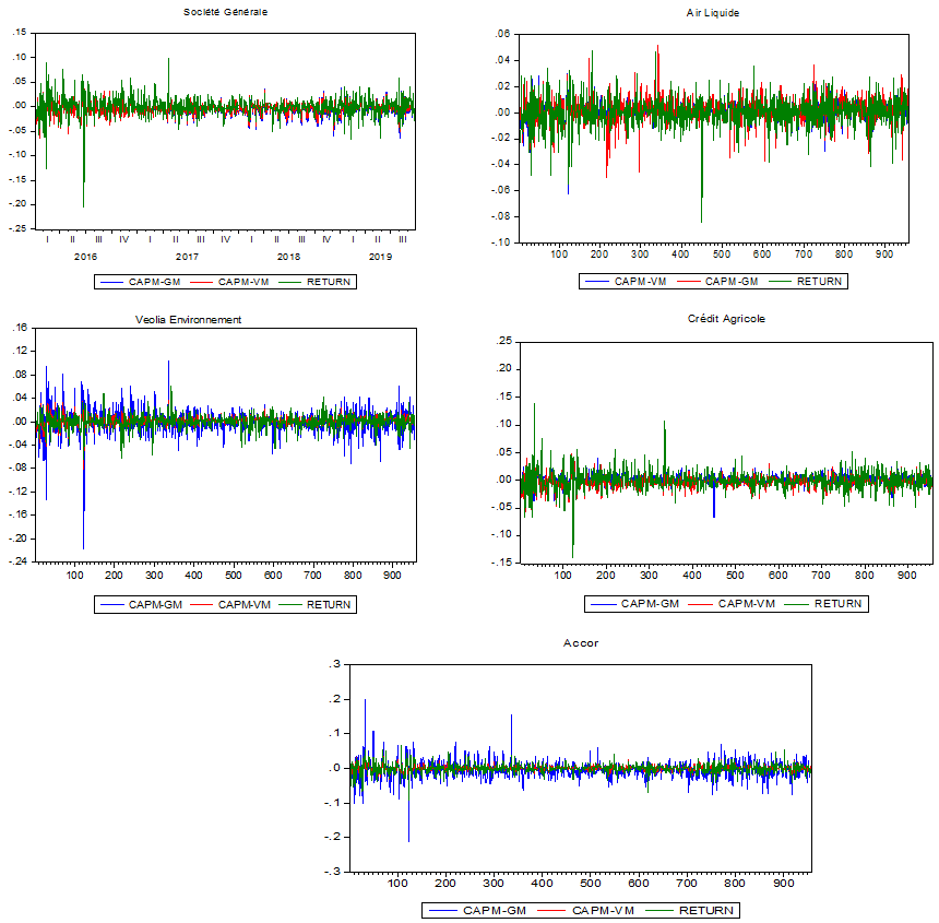
Figure-1. Graphical presentation of the returns estimated by the two CAPMs (Mean-Variance and Mean-Gini) and the real returns of each asset.

In Table 2, we have the descriptive statistics of the daily returns of each stock for the period from January 4, 2016 to September 27, 2019 estimated by the two models. We note that the estimates of the two models are divergent for each asset, which leads us to try to see which of the two models is close to the reality of asset returns and therefore the most predictive model in this study.

	CAPM-MV					CAPM-MG
Stocks	AC_PA	ACA_PA	AI_PA	GLE_PA	VIE_PA	AC_PA	ACA_PA	AI_PA	GLE_PA	VIE_PA
Mean	0.000448	-0.003027	0.001562	-0.004868	0.001732	-0.004185	0.002111	0.001963	-0.006063	-0.000821
Median	0.000580	-0.002834	0.001671	-0.004679	0.002026	-0.004725	0.002544	0.002488	-0.005970	-0.000972
Maximum	0.040292	0.054671	0.037038	0.060489	0.036815	0.200064	0.041172	0.052023	0.061984	0.103521
Minimum	-0.086814	-0.127774	-0.062169	-0.146186	-0.082324	-0.210945	-0.067479	-0.051668	-0.139514	-0.217645
Std. Dev.	0.009830	0.013553	0.008269	0.015411	0.008925	0.027303	0.009681	0.010284	0.016025	0.021467
Skewness	-0.774077	-0.837457	-0.450551	-0.821901	-1.057982	0.625983	-0.548418	-0.467482	-0.570909	-0.975677
Kurtosis	11.25824	12.45311	8.215742	12.28419	13.63626	14.24685	7.524051	6.790754	9.617944	17.04840
Jarque-Bera	2817.931	3678.985	1118.303	3548.520	4694.494	5111.692	864.9977	608.4886	1800.279	8029.847
Probability	0.000000	0.000000	0.000000	0.000000	0.000000	0.000000	0.000000	0.000000	0.000000	0.000000
Sum	0.429110	-2.900038	1.496196	-4.663272	1.659720	-4.009001	2.022122	1.880774	-5.808701	-0.786372
Sum Sq. Dev.	0.092466	0.175788	0.065443	0.227287	0.076230	0.713375	0.089687	0.101218	0.245749	0.441036
Observations	958	958	958	958	958	958	958	958	958	958

(c) Comparison of results: In order to see which of the two models is closer to reality, we compare the square sums of the differences between the value estimated by each model and the real return of each asset. Table 3 shows that the most appropriate model is that which presents the minimum difference with the real return on assets. Based on the results we have found that the CAPM-MV presents the minimum difference for assets, Société Générale (GLE.PA) and Credit Agricole (ACA.PA).On the contrary for the assets, Veolia Environnement (VIE.PA), Air Liquide (AI.PA) and Accor (AC. PA), the CAPM-MG is the model that presents the minimum difference compared with CAPM-MV.

Stocks	GLE.PA	VIE.PA	AI.PA	ACA.PA	AC.PA
CAPM-MV	0.63276014**	0.66356003	0.57821482	0.23379807**	0.40205256
CAPM-MG	0.9079052	0.47262724**	0.2825001**	0.28876372	0.30378474**

Note: ** Minimum of square sums of the differences between the value estimated by each model and the real return of each asset

5. Conclusion

As part of this study, we appreciated the contribution of the Mean-Gini model of Shalit and Yitzhaki (1984) to solve problems related to the valuation of financial assets and especially of assets that do not exhibit normal behavior. The empirical application on a sample of assets allowed us to obtain the following main results:

• The different series of returns of our stocks are volatile, leptokurtic and asymmetrical. They result in a rejection of the Jarque-Bera normality test. As a result, the distribution of daily asset returns differs from that of the normal distribution. On the basis of these observations, we opted for CAPM-MG since it makes no assumption on the distribution of the returns whereas the CAPM-MV is built on the assumption of normality of the returns what makes it inappropriate to reality financial market.
• The two valuation models (CAPM-MV and CAPM-MG) resulted in different results and deviations from the actual returns observed in the financial markets.
•  Finally, we emphasize that the results obtained confirm the relevance of the CAPM-MG model for the valuation of the financial assets in this study. However, this study remains to be applied to all of CAC40's financial assets and to emerging markets to test the validity of each model.

References

Agouram, J., & Lakhnati, G. (2015a). Mean-gini portfolio selection: Forecasting VaR using GARCH models in Moroccan financial market. Journal of Economics and International Finance, 7(3), 51-58.

Agouram, J., & Lakhnati, G. (2016). Mean-Gini and mean-extended gini portfolio selection: An empirical analysis. Risk Governance & Control: Financial Markets and Institutions, 6(3-1), 59-66.Available at: http://dx.doi.org/10.22495/rcgv6i3c1art7.

Agouram, J., & Lakhnati, G. (2015b). A comparative study of mean-variance and mean gini Portfolio selection using VaR and CVaR. Journal of Financial Risk Management, 4(2), 72-81.Available at: https://doi.org/10.4236/jfrm.2015.42007.

Bantz, R. (1981). The relationship between return and market values of common stock. Journal of Financial Economics, 9(1), 3-18.Available at: https://doi.org/10.21002/icmr.v8i1.5186.

Basu, S. (1977). Investment performance of common stocks in relation to their price-earnings ratios: A test of the efficient market hypothesis. The Journal of Finance, 32(3), 663-682.Available at: https://doi.org/10.1111/j.1540-6261.1977.tb01979.x.

Belimam, D., & Lakhnati, G. (2018). Beta, size and value factors in the Chinese stock returns. Paper presented at the In International Conference on Applied Economics. Springer, Cham.

Belimam, D., Tan, Y., & Lakhnati, G. (2018). An empirical comparison of asset-pricing models in the Shanghai A-share exchange market. Asia-Pacific Financial Markets, 25(3), 249-265.Available at: https://doi.org/10.1007/s10690-018-9247-4.

Bhandari, L. C. (1988). Debt/equity ratio and expected common stock returns: Empirical evidence. The Journal of Finance, 43(2), 507-528.Available at: https://doi.org/10.1111/j.1540-6261.1988.tb03952.x.

Black, F., Jensen, M. C., & Scholes, M. (1972). The capital asset pricing model: Some empirical tests. Studies in the Theory of Capital Markets, 81(3), 79-121.

Campbell, J. Y., & Cochrane, J. H. (2000). Explaining the poor performance of consumption-based asset pricing models. The Journal of Finance, 55(6), 2863-2878.Available at: https://doi.org/10.1111/0022-1082.00310.

Chan, K., & Chen, N.-F. (1991). Structural and return characteristics of small and large firms. The Journal of Finance, 46(4), 1467-1484.Available at: https://doi.org/10.1111/j.1540-6261.1991.tb04626.x.

Fama, E. F., & French, K. R. (1992). The cross-section of expected stock returns. The Journal of Finance, 47(2), 427-465.

Fama, E. F., & James, D. M. (1973). Risk, return, and equilibrium: Empirical tests. Journal of Political Economy, 81(3), 607-636.Available at: https://doi.org/10.1086/260061.

Fama, E. F., & French, K. R. (1993). Common risk factors in the returns on stocks and bonds. Journal of Financial Economics, 33, 3-56.Available at: https://doi.org/10.1016/0304-405x(93)90023-5.

Fama, E. F., & French, K. R. (2015). A five-factor asset pricing model. Journal of Financial Economics, 116(1), 1-22.

Fama, E. F., & French, K. R. (2016). Commodity futures prices: Some evidence on forecast power, premiums, and the theory of storage The World Scientific Handbook of Futures Markets (pp. 79-102): World Scientific.

Hansen, L. P., & Singleton, K. J. (1982). Generalized instrumental variables estimation of nonlinear rational expectations models. Econometrica, 50(5), 1269-1286.Available at: https://doi.org/10.2307/1911873.

Jegadeesh, N. (1990). Evidence of predictable behavior of security returns. The Journal of Finance, 45(3), 881-898.Available at: https://doi.org/10.1111/j.1540-6261.1990.tb05110.x.

Lintner, J. (1965). Security prices, risk, and maximal gains from diversification. The Journal of Finance, 20(4), 587-615.Available at: https://doi.org/10.1111/j.1540-6261.1965.tb02930.x.

Markowitz, H. (1952). Portfolio selection. The Journal of Finance, 7(1), 77-91.Available at: 10.2307/2975974.

Markowitz, H. (1952b). The utility of wealth. Journal of political Economy, 60(2), 151-158.

Markowitz, H. (1959). Portfolio selection: Efficient diversification of investments (Vol. 16). New York: John Wiley.

Mossin, J. (1966). Equilibrium in a capital asset market. Econometrica: Journal of the econometric society, 34(4), 768-783.Available at: https://doi.org/10.2307/1910098.

Parker, J. A., & Julliard, C. (2005). Consumption risk and the cross section of expected returns. Journal of political Economy, 113(1), 185-222.

Ross, S. A. (1976). The arbitrage theory of capital asset pricing. Journal of Economic Theory, 13(3), 341-360.Available at: 10.1016/0022-0531(76)90046-6.

Shalit, H., & Yitzhaki, S. (1984). Mean-Gini, portfolio theory, and the pricing of risky assets. The Journal of Finance, 39(5), 1449-1468.Available at: https://doi.org/10.1111/j.1540-6261.1984.tb04917.x.

Sharpe, W. F. (1964). Capital asset prices: A theory of market equilibrium under conditions of risk. The Journal of Finance, 19(3), 425-442.Available at: https://doi.org/10.1111/j.1540-6261.1964.tb02865.x.

Tobin, J. (1958). Estimation of relationships for limited dependent variables. Econometrica: Journal of the Econometric Society, 26(1), 24-36.Available at: https://doi.org/10.2307/1907382.

Yaşar, E. (2017). Comparison of CAPM, threefactor Fama-French model and five-factor Fama-French model for the Turkish stock market, Financial Management from an Emerging Market Perspective, Guray Kucukkocaoglu and Soner Gokten, IntechOpen.Available at: 10.5772/intechopen.70867. Retrieved from: https://www.intechopen.com/books/financial-management-from-an-emerging-market-perspective/comparison-of-capm-three-factor-fama-french-model-and-five-factor-fama-french-model-for-the-turkish-.

Yitzhaki, S. (1982). Stochastic dominance, mean variance, and Gini's mean difference. The American Economic Review, 72(1), 178-185.

Yitzhaki, S. (1983). On an extension of the Gini inequality index. International Economic Review, 24(3), 6-17.

---

Footnote: