Impact of Shocks on the Balance of Payment Evidence via MGARCH from Sudan
Khalafalla Ahmed Mohamed Arabi1
1Professor of Econometrics and Social Statistics College of Business, King Khalid University, Saudi Arabia. |
AbstractThis research investigates the effects of own shocks on the Sudanese balance of payment (BOP) and shocks from other variables. The model encompasses seven variables that have long-term relationship with each other i.e. ratio of balance of payments to GDP (BOPR), economic growth proxied by per capita GDP (Q), real effective exchange rate (REER), budget deficit ratio to GDP (BUDR), monetization (MNT), inflation rate (INF), and unemployment rate (UR). We use a multivariate generalized autoregressive conditional heteroscedasticity model (MGARVH) for estimation. We chose t distribution because residuals are not multivariate normal. All estimates are highly significant and positive. Positive ARCH effects suggest that a shock to the ith variable has positive effects on all variable covariances in the next period. The multiplication of own shocks by the cross shocks discloses that the covariance of the balance of payments and the inflation rate is the largest contrary to the smallest amount covariance of the balance of payments and the fiscal deficit. The positive estimates of the cross terms capture linkages, the transformation of shocks and volatility spillover effects point toward model variables integration. Covariance stationary test indicates multidirectional volatility spillover runs from single variable to the other variables. Dynamic conditional correlation (DCC) reveals a strong correlation of the variable model comprising both signs. We recommend that policymakers when formulating macroeconomic policies should consider the linkages between these variables taking Kaldor magic square as a guideline. . |
Licensed: |
|
Keywords: |
Funding: This study received no specific financial support. |
Competing Interests: The author declares that there are no conflicts of interests regarding the publication of this paper. |
1. Introduction
The rationale for foreign trade stems from two situations: importing goods and services, that the receiving country cannot produce and supply or production and supplies are not enough. Alternatively, despite the capability, imports are necessitated by the transfer of production abroad or ceased production due to lack of competitiveness. Moreover, goods and services may be cheaper, of greater variety, or better quality and design. Countries are classified as a creditor nation if has a surplus in the balance of payments and debtor otherwise. Persistence deficit in the balance of payments may result from the excessive outflow of capital, or imports. The appropriate measure to control import is restricting their number of value. On the other hand, increase their prices via imposing import duties. The country can subside or reduce taxes on exports. For fear that these two policies are constrained; monetary policy can play a significant role in reducing the deficit through an increase in interest rates, or open market operations, or direct the banks to deposit a certain amount of their fund with the central bank (Sherlock & Reuvid, 2008) that is reduction of spending power directly or indirectly. Another measure to tackle the deficit of the balance of payments is the devaluation of the local currency to make export cheaper and competitive while pushing import prices up.
The balance of payment mirrors whether a country is technology advances, its equilibriums make known sound economic position n even though a distortion replicates unsatisfactory position (Azra, 2015). The balance of payments relates to the fundamental economic variables. The magic square of economic policy by Kaldor links it to major economic policy goals, i.e. high and steadies GDP growth, a high employment rate, a low inflation rate, and a balanced current account.
Some researchers have engaged in the issue of the Sudanese balance of payments using a single equation and vector error correction as an analytical tool of which (Yousif & Musa, 2017). This research aims to investigate the effects of its own shocks on the Sudanese balance of payment (BOP) and shocks from other variables. This research specifies the MGARCH model as an estimation technique containing seven variables aims at tracing the effects of shocks on the balance of payments. The problem of this research is to answer the following questions. Are there linkages between the model variable? What are the types of shock that influence the balance of payment? What are the directions of shocks and volatility spillover?
The structure of this paper consists of six sections. The first section introduces the topic followed by a literature review in section two, then a theoretical background in section 3. Section 4 presents empirical analysis followed by discussion in the fifth section, and finally the conclusion
2. Literature Review
Empirical research has identified many internal and external factors that affect the behavior of the balance of payments. Internal factors include inflation rate, exchange rate, money supply, real gross domestic product, interest rate, fiscal balance, and unemployment rate. However, the external factors comprise foreign direct investment,
Zhang (2017) was interested in factors determining the surplus in the current account and capital account in China. His research attributed this double surplus largely to the inflow of foreign direct investment to the Chinese economy. Kennedy (2013) through investigating the long-run determinants of the balance of payment dynamics in Kenya during the period 1963 – 2012 and Muharremi (2015) for the Western Balkan countries reached the same conclusion.
Yousif and Musa (2017) studied the determinants of the Sudanese balance of payments during the period 1980 – 2016 to conclude that four variables are the most influential on the balance of payments that is external debt, exchange rate, gross domestic product, and inflation.
Geetha, Aghalya, and Gayathiri (2017) attribute imbalance of the payment to inequality between export and import. The inflation rate is the most factors that disturb the balance of payments by means of higher prices of domestic goods leading to export decline hence causes current account decrease.
Anulika (2016) set up that tariff, indirect tax and interest as a proxy for non- tariff, exchange rate, money supply, and export affect the Nigerian balance of payments (BOP) via ordinary least square (OLS) method. The result shows that the indirect tax, export and exchange rate satisfy the economic a priori expectation while the interest rate and money supply negates the a priori expectation.
Blecker (2016) focused on the significance of the real exchange rate (relative prices) on long-run growth and hence the balance of payments.
Azra (2015) declares via a bound test that there exists a negative and stable long-run relationship of the balance of payments to the real exchange rate, interest rate, and fiscal balance, while real GDP moves the BOP in the positive direction in both long and short run. The money supply cast a positive influence on the BOP in the short run but a negative effect in the long term.
Kandil and Greene (2015) established that Real GDP growth and real effective exchange rate (REER) appreciation appear co-integrated with the current and financial accounts of the U.S. balance of payments. On this basis, we estimate reduced form equations showing that expected changes and shocks to real GDP, the REER, energy prices, and growth in emerging market economies and other industrial countries explain much of the short-term variation in the U.S. current account balance, with the balance worsening as real GDP, the REER, and to a lesser extent, energy prices increase. In addition, the financial balance improves with real growth and an increase in the oil price, while stock market prices affect the composition of capital inflows.
Edmore (2015) empirical results indicate that the determinants of the balance of payments are a foreign direct investment, Inflation, drought, money supply, and external debt in Zimbabwe.
Kennedy (2013) examined the long-run determinants of the balance of payment dynamics in Kenya between 1963 and 2012, using cointegration and error correction mechanism. The study uses annual time series data for Kenya. Results show that the level of trade balance, exchange rate movement and foreign direct investment inflow could cause balance of payments fluctuations. The investigation further reveals that FDI and Exchange rates are the main determinants of the balance of payments
Gureech (2012) assessed the determinants of the balance of payment performance in Kenya using time-series data for period the1975 – 2012. He found the relationship between the balance of payments, money supply, exchange rate, real interest rate, terms of trade, the openness of the economy, gross capital formation and political instability via the VAR model. Ozturk and Acaravci (2009) tested the validity of Thirlwall’s Law in Turkey during the period of 1980:1-2006:4 using an Autoregressive Distributed Lag (ARDL) Bounds testing approach. The empirical results reveal the cointegration of import with relative price and income. The difference between the equilibrium and actual economic growth rates are small. Nevertheless, results from regressions of equilibrium growth rates indicate that the Thirlwall’s law does not hold for Turkey. Razmi (2005) applies the Balance of Payments Constrained Growth (BPCG) model to India employing Johansen’s cointegration technique and vector error correction to estimate trade parameters. He found the average growth rates predicted by various forms of the BPCG hypothesis to be close to the actual average growth rate over the period 1950-1999, although individual decades display substantial deviations.
Alawattage (2001) examines the effectiveness of the exchange rate policy of Sri Lanka in achieving external competitiveness since the liberalization of the economy in 1977. The conventional two-country trade model that explains the traditional approach to Balance of Payment (BOP) was applied using quarterly data covering the period of 1978:1 to 2000:4. Results reveal that the Real Effective Exchange Rate (REER) does not have a significant impact on improving the Trade Balance (TB) particularly in the short run implying a blurred J-Curve phenomenon. Even though the cointegration tests disclose that there is a long run relationship between TB and the REER it shows a very marginal impact in improving TB in long run.
Thirlwall (1979) postulates are that the ultimate constraint on growth is either a shortage of foreign exchange or the growth of exports to which factor supplies can adapt. Changes in growth equilibrate the balance of payments, not changes in relative prices in international trade.
3. Theoretical Background
The elasticity approach determines the relationship between the balance of payments and exchange rate. The degree of elasticity determines the stability of the foreign exchange market equilibrium. Similarly, the magnitude of the absorption relative to national income determines the magnitude of the balance of payments in harmony with the devaluation of local currency and inflation. In the same fashion, the BOP-constrained growth model assumes that in the long term, no country can grow faster than the rate consistent with balance on the current account, unless it can finance ever-growing deficits from external sources. Much borrowing specifically short-term will induce capital flight, triggering the collapse of the exchange rate. Inflation is usually is considered as monitory phenomenon a large amount of money chases few goods. This may result in a shortage of goods and services domestically, resulting in increased drawings from banks increase in money supply and inflation. If extreme deficit it may result in devaluation (Svensson & Razin, 1983).
The ratio of broad money (MS) to nominal GDP i.e. degree of monetization and financial deepening are two faces of the same coin. Per capita GDP influences monetization (Lin & Wang, 2005). Fiscal deficit induces government borrowing via bonds causes the interest rate to rise, lowering private consumption and investment, therefore output. The government can print money increasing the monetary base and money supply, leading to higher credit supply, and then higher inflation (Nguyen, 2014). The accumulation of foreign exchange reserves because of the surplus in the balance of payment will influence the monetary policy by increasing the money supply. Therefore, excessive foreign exchange reserves are the reason to CPI increase.
Kaldor magic square relates a high GDP growth to low employment rate, zero inflation rate, and a balanced current account. The interest rate, exchange rate, and import prices are the main channels that transmit the effects of money supply on economic growth, unemployment, inflation, and balance of payments. Expansionary monitory policy raises the price level, lowers real interest rate, which has two contradicting effects. It spurs investment leading to the creation of more job and reduction in unemployment accompanied by increased economic output and growth. An adverse effect on foreign capital is pushing it outside the country. Deposits in local currency become less attractive compared to foreign matching part, therefore, the relative size of latter to total deposits increases lead eventually to the reduction of the exchange rate. Capital flight renders local-currency deposits become less attractive than foreign currency, increasing the relative size of the latter to total deposits in the banking system, which eventually leads to a lower exchange rate, the US will, rising import prices and lower export prices lead the balance of trade to equilibrium (Ratoul & Croush, 2014).
4. Empirical Results
4.1. Data Set
Data about the variables are included in the Table 1 for the period 1960 – 2017. The start year represents the setting up of the central bank of Sudan.
| Variable | Acronym | Source | |
| Balance of Payments | BOP | Million SDG | CBoS* |
| Gross Domestic Product | GDP | Million SDG | CBoS* |
| Broad Money Supply | MS | Million SDG | CBoS* |
| Real Effective Exchange Rate | REER | Million SDG | World Bank |
| Gross Domestic Product | GDP | Million SDG | CBS** |
| Per capita GDP | Q | Million SDG | CBoS* |
| Inflation Rate | INF | Rate | CBoS* |
| Unemployment Rate | UR | Rate | ILO*** |
| Monetization | MNT | MS/GDP | Constructed |
| Budget Deficit ratio to GDP | BUDR | Rate | Constructed |
| * Central Bank of Sudan; **Central Bureau of Statistics; ***International Labour Organization. |
4.2. Diagnostic Tests
Annex (1) displays results of unit root tests. The balance of payments ratio to GDP (BOPR), per capita (Q), inflation rate (INF) are stationary of order of one i.e. I(1), while real effective exchange rate (REER), monetization (MNT), budget deficit ratio to GDP (BUDR), and unemployment rate (UR) are stationary. Annex (2) reveals that there are five cointegrating equations i.e. there is a long-run relationship among the seven variables and at simultaneously avoiding the risk of spurious regression is over.
4.3. The Estimated Model
The main objective of multivariate GARCH (MARCH) is to estimate the variance and covariances of the error terms in an autoregressive form. These models allow a variance to vary over time (time-varying). An (i,i) represents own shocks; A(i,j) captures ARCH effects of the own shocks, B(j,j) is the shocks from other variables; and B(i,j) the rate of shock decay. Covariance stationary test A(i,i) + B(j,j) indicates no multidirectional volatility spillover runs from a single variable to the other variables. Cross terms capture linkages, the transformation of shocks and volatility spillover effects to indicate model variables integration (Mad'ar, 2014). With regard to the mean equations, a positive A(i,i)A(i,j) and A(i,j) suggest a shock to the ith variable has positive effects on all variable covariances in the next period. Concerning the variance and covariance a positive B(j,j) B(i,j) means an increase in the ith variable has a positive effect on the variables covariances in the next period (Tsuji, 2017).
| Diagonal VECH | Coefficient |
Probability |
BEKK | Coefficient |
Probability |
| C(1) | -1.16373 |
0.03090 |
C(1) | -2.53143 |
0.00770 |
| C(2) | 107.5122 |
0.00000 |
C(2) | 108.6252 |
0.00000 |
| C(3) | 539.1539 |
0.00000 |
C(3) | 496.6257 |
0.00000 |
| C(4) | 22.5284 |
0.00000 |
C(4) | 19.59252 |
0.00000 |
| C(5) | -4.18472 |
0.00000 |
C(5) | -3.71761 |
0.00000 |
| C(6) | 7.016273 |
0.00000 |
C(6) | -6.71818 |
0.00710 |
| C(7) | 11.67473 |
0.00000 |
C(7) | 13.24437 |
0.00000 |
The estimated coefficients of the mean equation are highly significantly different from zero, which indicate that lagged values of all model variables are substantial determinants of current values. There are slight differences between the estimates via DVECH and BEKK.
| Diagonal VECH | Coefficient |
Probability |
BEKK | Coefficient |
Probability |
| M | 0.184102 |
0.00020 |
M | 0.072312 |
0.00010 |
| A1(1,1) | 0.290129 |
0.00050 |
A1(1,1) | 0.539212 |
0.00000 |
| A1(1,2) | 0.527128 |
0.00030 |
|||
| A1(1,3) | 0.727857 |
0.00000 |
|||
| A1(1,4) | 0.447858 |
0.00040 |
|||
| A1(1,5) | 0.141291 |
0.00560 |
|||
| A1(1,6) | 1.553021 |
0.00000 |
|||
| A1(1,7) | 0.635181 |
0.00030 |
|||
| A1(2,2) | 0.957725 |
0.00340 |
A1(2,2) | 1.030399 |
0.00000 |
| A1(2,3) | 1.322424 |
0.00060 |
|||
| A1(2,4) | 0.813702 |
0.00540 |
|||
| A1(2,5) | 0.256709 |
0.00740 |
|||
| A1(2,6) | 2.821644 |
0.00000 |
|||
| A1(2,7) | 1.154043 |
0.00250 |
|||
| A1(3,3) | 1.825999 |
0.00020 |
A1(3,3) | 0.984074 |
0.00000 |
| A1(3,4) | 1.123557 |
0.00230 |
|||
| A1(3,5) | 0.354463 |
0.00180 |
|||
| A1(3,6) | 3.896118 |
0.00000 |
|||
| A1(3,7) | 1.5935 |
0.00110 |
|||
| A1(4,4) | 0.691337 |
0.01340 |
A1(4,4) | 0.459501 |
0.00010 |
| A1(4,5) | 0.218105 |
0.00950 |
|||
| A1(4,6) | 2.397323 |
0.00000 |
|||
| A1(4,7) | 0.980498 |
0.00730 |
|||
| A1(5,5) | 0.068808 |
0.06590 |
A1(5,5) | 0.154334 |
0.04570 |
| A1(5,6) | 0.756314 |
0.00060 |
|||
| A1(5,7) | 0.30933 |
0.00670 |
|||
| A1(6,6) | 8.31311 |
0.00000 |
A1(6,6) | 1.322911 |
0.00000 |
| A1(6,7) | 3.400036 |
0.00000 |
|||
| A1(7,7) | 1.390604 |
0.00930 |
A1(7,7) | 0.858574 |
0.00000 |
| B1(1,1) | 0.975712 |
0.00000 |
B1(1,1) | 0.965387 |
0.00000 |
| B1(1,2) | 0.890378 |
0.00000 |
|||
| B1(1,3) | 0.730799 |
0.00000 |
|||
| B1(1,4) | 0.854546 |
0.00000 |
|||
| B1(1,5) | 0.95676 |
0.00000 |
|||
| B1(1,6) | 0.229583 |
0.00000 |
|||
| B1(1,7) | 0.675447 |
0.00000 |
|||
| B1(2,2) | 0.812507 |
0.00000 |
B1(2,2) | 0.89418 |
0.00000 |
| B1(2,3) | 0.666885 |
0.00000 |
|||
| B1(2,4) | 0.779809 |
0.00000 |
|||
| B1(2,5) | 0.873083 |
0.00000 |
|||
| B1(2,6) | 0.209504 |
0.00000 |
|||
| B1(2,7) | 0.616374 |
0.00000 |
|||
| B1(3,3) | 0.547361 |
0.00000 |
0.798285 |
0.00000 |
|
| B1(3,4) | 0.640047 |
0.00000 |
|||
| B1(3,5) | 0.716604 |
0.00000 |
|||
| B1(3,6) | 0.171955 |
0.00000 |
|||
| B1(3,7) | 0.505904 |
0.00000 |
|||
| B1(4,4) | 0.748426 |
0.00000 |
B1(4,4) | 0.934079 |
0.00000 |
| B1(4,5) | 0.837947 |
0.00000 |
|||
| B1(4,6) | 0.201072 |
0.00000 |
|||
| B1(4,7) | 0.591569 |
0.00000 |
|||
| B1(5,5) | 0.938176 |
0.00000 |
B1(5,5) | 0.979307 |
0.00000 |
| B1(5,6) | 0.225123 |
0.00000 |
|||
| B1(5,7) | 0.662328 |
0.00000 |
|||
| B1(6,6) | 0.05402 |
0.00030 |
B1(6,6) | 0.408894 |
0.00000 |
| B1(6,7) | 0.158931 |
0.00000 |
|||
| B1(7,7) | 0.467586 |
0.00000 |
B1(7,7) | 0.680069 |
0.00000 |
The positive ARCH effects A(i,j) produced by the model means that the shocks from the previous period have a profound effect on the current period. All own shocks A(i,i) are positive and significantly different from zero. The fiscal deficit own shock was the smallest among all own shock followed by the balance of payments. The highest own shock was that for inflation rate trailed by per capita (economic growth). The VECH estimate A(1,1) is almost twice as that of BEKK, concerning another variable however there are slight differences among the estimates of the two approaches. Shocks resulting from the product A(i,i)A(i,j) represents the effect of the current own shock on the covariance of the ith variable with the jth variable in the next period. Taking the product of the first variable (balance of payments) with the covariances of other variable offers the following (0.15, 0.51 1.32, 0.31, 0.01, 12.91, and 0.88) to reach the conclusion that the covariance of balance of payments and inflation rate is the maximum contrary to the minimum covariance of balance of payments and the fiscal deficit. The same approach is applicable to other products.
The positive effects of variances and covariance B(j,j)B(i,j) means an increase in one variable variance has a positive effect on the covariance in the next period. For instance, an increase in the variance of the balance of payments increases the covariances of other variables in the next period. The results is as follows: (0.87, 0.72, 0.40, 0.64, 0.90, 0.01, and 0.11).The conclusion is that the covariance of the balance of payments and the real effective exchange rate is the biggest contrary to the least covariance of the balance of payments and the inflation rate. The same approach is applicable to other products.
Concerning the shocks from other variables, they are all positive whereas inflation reveals the leading shock tracked by the unemployment rate. The rate of shock decay of five model variables on the balance of payments i.e. real effective exchange, per capita, monetization, fiscal deficit, and the unemployment rate is positive and similarly high, while the inflation rate has the least rate of shock decay not only on the balance of payments but on all model variables. This means that shocks of the aforementioned five variables depleting quickly compared to the inflation rate, which takes almost three times more to vanish. According to the covariance stationary test, the only variable that has a sum of own shock and shocks from other variables is the monetization A(4,4) + B(4,4) = 0.8) indicates no multidirectional volatility spillover runs from a single variable to the other variables. While the other sum is greater than one indicting multidimensional spillover from a single variable to the other variables.4.4. Ordinary and Dynamic Conditional Correlation
Annex (3) presents results of ordinary correlation whereas the balance of payments correlates negatively with per capita GDP, real effective exchange rate and monetization correlate with monetization, negative correlation between per capita and inflation and the unemployment rate, which in turn correlates with inflation. The picture is different when it comes to conditional correlation. Negative and strong conditional correlation is present among most model variables (annex 4). Figure 1 point toward a breakpoint at the year 1992 that witnessed the announcement of economic liberalization policy that has profound adverse effects on macroeconomic variables in general, exchange rate, inflation, the balance of payments, fiscal deficit and money supply specifically.
5. Discussion
The covariance stationary test indicates multidirectional volatility spillover runs from a single variable to the other variables except for the inflation rate. The positive estimates of the cross terms capture linkages, the transformation of shocks and volatility spillover effects point to model variables integration. The own shock of the balance of payment is relatively low compared to other variables' own shocks. ARCH effects reflect the excessive influence of inflation on the balance of payments relative to the other variables' influence. Shocks from other variables on the balance of payment are slightly more than the rate of the shock decay rate of the fiscal deficit tracked by real effective exchange rate, monetization, per capita GDP, unemployment rate and finally the inflation rate which indicate lasting influence.
The Sudanese balance of payments been running in deficit since 1961 except a few years with a mean ratio to GDP (-2.96%). Primary goods typically agricultural and minerals constitute 90 percent of goods exports although the country has no control on their prices that lacks the ability to compete in external markets, In addition, export of agricultural goods has always been under the mercy of weather conditions (poor harvest) and external demand. Politics has tremendous effects on foreign trade as manifest in economic sanctions. The demand for import has been growing despite efforts to curb it by trade policies such as licensing, quotas, currency devaluation etc. One of the main causes of the current account deficit is the government purchases of vehicles and equipment for the central and state governments, augmented by debt service payments and transfers to diplomatic missions all over the world. A series of devaluation has started in September 1978 and has been continuing up today as a tool to reduce the deficit of the balance of payment as IMF and World Bank advocate. The real growth rate has not been consistent with the current account as Thirlwall (1979) postulates, causing accumulation of total debt and collapse of the exchange rate.
The application of Kaldor magic square on Sudanese economy necessitates comparing the actual values with the target ones. The average balance of payments ratio to GDP is equal to -2.96 percent throughout the sample period since the balance of payments (the average current account ratio to GDP is equal to -3.77 percent) have been realizing few surpluses. The average unemployment rate is equal to 12.7 percent; the mean of the inflation rate is equal to 27.96; the real growth rate is equal to 3.86 and money supply growth rate is equal to 32.93 percent (the annual target is 19 percent). Comparing these figures with the target 5 percent growth rate; zero inflation rate; zero unemployment rate; and balance of payment greater than or equal to zero it is obvious that the effectiveness of the monitory policy is of great doubt. As these peaks move into the magic square along the axes, the economic situation becomes more difficult.
6. Conclusion
The main objective of this research is to capture multidirectional volatility spillover runs from the balance of payment, real effective exchange rate, growth, monetization, fiscal deficit, inflation, and unemployment rate via multivariate GARCH (DVECH and BEKK). All estimates of own shocks shock from other variables, and cross terms are positive and significant capturing linkages, the transformation of shocks and volatility spillover effects hence model variables integration.
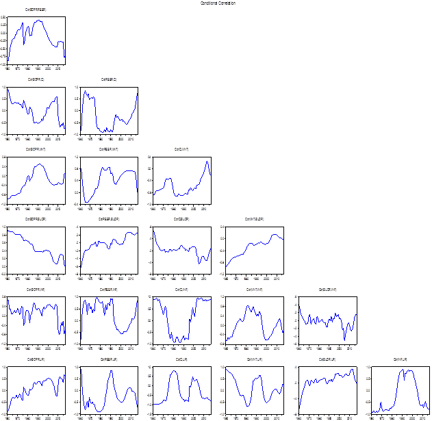
Figure-1. Dynamic Conditional Correlation.
References
Alawattage, U. P. (2001). Exchange rate, competitiveness, and balance of payment performance. Retrieved from https://ss.sljol.info/article/10.4038/ss.v35i1.1234/galley/.../download/.
Anulika, A. (2016). The balance of payments and policies that affects its positioning in Nigeria MPRA Paper No. 74841, posted 1 November 2016 15:09 UTC. Retrieved from https://mpra.ub.uni-muenchen.de/74841/.
Azra, F. (2015). Synthetic biology: Generation of new GFP variants with improved characteristics. NTNU.
Blecker, R. A. (2016). The debate over ‘Thirlwall’s law’: balance-of-payments-constrained growth reconsidered. Retrieved from s2.american.edu/blecker/www/research/Blecker-BPCG-debate-revised0816.pdf.
Edmore, M. (2015). Determinants of balance of payment dynamics in Zimbabwe (1981 – 2012) great Zimbabwe University a dissertation submitted in partial fulfilment of the requirement of a bachelor of commerce honours degree in economics. Retrieved from https://www.academia.edu/31308928/DETERMINANTS_OF_BALANCE_OF_PAYMENTS_DYNAMICS_IN_ZIMBABWE.
Geetha, R. K., Aghalya, V., & Gayathiri, G. G. (2017). The balance of payments problems of developing countries with special reference to India SSRG. International Journal of Economics and Management Studies, Special Issue, 19-25.
Gureech, M. I. (2012). The determinants of the balance of payments master of arts in economic policy management of the University of Nairobi, Kenya. Retrieved from http://erepository.uonbi.ac.ke/bitstream/handle/11295/76538/Mabior%20_The%20determinants%20of%20balance%20of%20payments%20performance%20in%20Kenya.pdf?sequence=3&isAllowed=y.
Kandil, M., & Greene, J. (2015). Impact of cyclical factors on U.S. balance of payments. International Journal of Business, Economics, and Law, 6(3), 28-48.
Kennedy, O. (2013). Determinants of balance of payments in Kenya. European Scientific Journal, 9(16), 112-134.
Lin, M.-Y., & Wang, J.-S. (2005). Foreign exchange reserve and inflation: An empirical study of five East Asian economies. Retrieved from http://citeseerx.ist.psu.edu/viewdoc/download?doi=10.1.1.583.6429&rep=rep1&type=pdf.
Mad'ar, M. M. (2014). Multivariate GARCH. Retrieved from https://www.google.com.sa/search?q=Mad%27ar%2C+Mgr.+Milan+(2014)+Multivariate+GARCH&oq=Mad%27ar%2C+Mgr.+Milan+(2014)+Multivariate+GARCH&aqs=chrome..69i57.2334j0j8&sourceid=chrome&ie=UTF-8.
Muharremi, T. I. (2015). Factors affecting current account in the balance of payments of selected Western Balkan countries. Journal of Accounting and Management, 5(3), 61-68.
Nguyen, T. D. (2014). Impact of government spending on inflation in Asian emerging economies: Evidence from India, Vietnam, and Indonesia. Retrieved from http://encuentros.alde.es/anteriores/xviieea/trabajos/d/pdf/214.pdf.
Ozturk, I., & Acaravci, A. (2009). On the causality between tourism growth and economic growth: Empirical evidence from Turkey. Transylvanian Review of Administrative Sciences, 5(25), 73-81.
Ratoul, M., & Croush, S. (2014). Assessment of the effectiveness of monitory policy in Arab Economic Research Issueealizing Kador Magic Square in Algeria during the period (2000 – 2010). Arab Economic Research Issue, 66.
Razmi, A. (2005). Balance-of-payments-constrained growth model: the case of India. Journal of Post Keynesian Economics, 27(4), 655-687.
Sherlock, J., & Reuvid, J. (2008). The handbook of international trade a guide to the principles and practice of export: GMB Publishing Ltd.
Svensson, L. E. O., & Razin, A. (1983). The terms of trade and the current account: The Harberger-Laursen-Metzler effect. Journal of Political Economy, 91(1), 97–125.
Thirlwall, A. P. (1979). The balance of payments constraint as an explanation of international growth rate differences. Banca Nazionale del Lavoro Quarterly Review, 32(128), 45-53.
Tsuji. (2017). How can we interpret the estimates of the full BEKK model with asymmetry? The case of French and German stock returns. Business and Economic Research, 7(2), 342-351.
Yousif, F. M. K., & Musa, E. M. E. (2017). Edelweiss. Applied Science and Technology, 2(1), 41-45.
Zhang, B. (2017). The causes and effects of China’s double surplus of balance of payments—based on the study of FDI inflow in 1993-2012. Open Journal of Social Sciences, 5, 1-15. Available at: 10.4236/jss.2017.55001.
Annex
Annex-1. Unit Test
| Augmented Dickey-Fuller | Philip-Peron | |||||
| Variable | Level |
Ist Diff. |
2ND Diff. |
Level |
Ist Diff. |
2ND Diff. |
| BOPR | -0.62 |
-2.74** |
-4.19*** |
|||
| REER | -3.45*** |
-3.3*** |
||||
| Q | -0.03 |
-8.19*** |
0.08 |
-8.21*** |
||
| INF | 2.41 |
-10.55*** |
-2.39 |
-10.27*** |
||
| MNT | -3.53** |
1.93 |
-5.24*** |
|||
| BUDR | -5.39** |
-2.63* |
||||
| UR | -2.92*** |
-2.73*** |
||||
Annex-2. Cointegration Test
| Hypothesized | Trace |
0.05 |
|||||||
| No. of CE(s) | Eigenvalue |
Statistic |
Critical Value |
||||||
| None * | 0.747711 |
221.2674 |
125.6154 |
||||||
| At most 1 * | 0.561769 |
144.1454 |
95.75366 |
||||||
| At most 2 * | 0.524172 |
97.94497 |
69.81889 |
||||||
| At most 3 * | 0.402396 |
56.35384 |
47.85613 |
||||||
| At most 4 | 0.309774 |
27.5235 |
29.79707 |
||||||
| At most 5 | 0.111681 |
6.762268 |
15.49471 |
||||||
| At most 6 | 0.002327 |
0.130485 |
3.841466 |
||||||
| Annex-3. Covariance Analysis: Ordinary Date: 11/10/18 Time: 13:54 Sample: 1960 2017 Included observations: 58 Balanced sample (listwise missing value deletion) Correlation |
|||||||||
| Probability | BOPR |
REER |
Q |
MNT |
BUDR |
INF |
|||
| BOPR | 1 |
||||||||
| REER | -0.1990 |
1 |
|||||||
0.1342 |
----- |
||||||||
| Q | -0.5531 |
-0.0656 |
1 |
||||||
0.0000 |
0.6246 |
----- |
|||||||
| MNT | -0.0009 |
0.46756 |
-0.464 |
1 |
|||||
0.995 |
0.0002 |
0.0002 |
----- |
||||||
| BUDR | 0.02706 |
0.17445 |
-0.037 |
-0.099 |
1 |
||||
0.8402 |
0.1903 |
0.7852 |
0.4599 |
----- |
|||||
| INF | 0.1129 |
0.1352 |
-0.408 |
0.35897 |
0.198 |
1 |
|||
0.3985 |
0.3115 |
0.0015 |
0.0057 |
0.1363 |
----- |
||||
| UR | -0.0009 |
-0.0071 |
-0.280 |
0.32463 |
-0.147 |
0.59185 |
|||
0.9944 |
0.9579 |
0.0331 |
0.0129 |
0.2725 |
0.0000 |
||||
Annex-4. Conditional Correlation
BOPR |
REER |
Q |
MNT |
BUDR |
INF |
UR |
1.00 |
-0.82 |
0.71 |
-0.92 |
0.96 |
-0.53 |
-0.77 |
-0.82 |
1.00 |
-0.49 |
0.71 |
-0.66 |
0.71 |
0.70 |
0.71 |
-0.49 |
1.00 |
-0.92 |
0.64 |
-0.74 |
-0.93 |
-0.92 |
0.71 |
-0.92 |
1.00 |
-0.87 |
0.69 |
0.94 |
0.96 |
-0.66 |
0.64 |
-0.87 |
1.00 |
-0.32 |
-0.67 |
-0.53 |
0.71 |
-0.74 |
0.69 |
-0.32 |
1.00 |
0.81 |
-0.77 |
0.70 |
-0.93 |
0.94 |
-0.67 |
0.81 |
1.00 |