Nexus between Remittance, Nonperforming Loan, Money Supply, and Financial Volatility: An Application of ARDL
Md. Qamruzzaman1*
Ananda Bardhan2
Summatun Nasya3
1Associate Professor, School of Business and Economics, United International University, Dhaka, Bangladesh. |
AbstractThe motivation of the study is to investigate the nexus between Remittance, Nonperforming loan, Money supply, and finical volatility for the period from 1976 to 2017. To do so, study apply unit root test for determining variables order of integration, Lag length criteria test to select optimal lag for empirical test and long-run cointegration test i.e. Autoregressive Distributed Lagged (ARDL). Referring to unit root tests, it is apparent that variables established integration in mixed order i.e. few variables are stationary at level and few variable are at first difference. The results of Bound testing ascertain that the presence of long-run association between financial volatility and selected macro fundaments. Referring to the long-term model estimation, it is palpable that magnitudes from macro fundaments to financial volatility established that money supply in the economy is responsible for financial instability on the other hand, remittance and financial development play critical role in maintaining financial stability in the economy. |
Licensed: |
|
Keywords: JEL Classification |
|
Received: 25 August 2020 |
|
| (* Corresponding Author) |
Funding: This study received no specific financial support. |
Competing Interests: The authors declare that they have no competing interests. |
1. Background of the Study
In the last decade, Bangladesh has successfully retained economic growth although the global economy faced fluctuations. The increased GDP is evidence of this successful economic growth in Bangladesh. No matter whether a country is developed or developing, the financial industry treated as the backbone of the overall economy of a country. Though Bangladesh is facing an upward economic growth, the financial industry of Bangladesh considered the weakest part of this economy. A huge amount of remittance inflow, strong RMG sector, highly efficient agricultural sector is the main reasons for this continuous economic growth. On the other hand, even if after passing the 48 years of independence, Bangladesh is still searching for an efficient; reliable; trustworthy; strong and structured capital market.
After independence, the Dhaka Stock Exchange started its functions properly from 1976. Until 1996 when the Bangladesh stock market faced one of the biggest crashes, there were controllable and moderate fluctuations in the market. By 2006, the market started going upward again, when some profitable government companies and multinational companies enlisted in the stock market. However, the highest level of fluctuations or vulnerability in the stock market started from the very beginning of the last decade.
During the period of 2009-10, the stock market maintained a strong bullish trend with average turnover was almost 2818 million BDT daily. Even the highest daily turnover was almost 32500 million BDT, which was beyond imaginations. At the end of 2010, this bullish trend turned into an erratic bubble. The broad index touched its historic high with 8919 and market capitalization became 35% as a percentage of GDP. Obviously, if there exists an inevitable upward turn, the market would soon face an inevitable downturn and in reality, downturn started from 2011 and by April 2013, the index came down to 3610 (Arif, 2018). A huge number of investors both individuals and companies lose a huge amount of investment. Different reasons were behind that, such as different swindles from big companies, political bad influence, lack of investment knowledge and so on. From that period, investors totally lose confidence in the stock market. This is the reason why there was a start of high stock price volatility in Bangladesh for the last few years. Even it seen that one day there is an upward trend and the next day, there is a downward trend. After taking different steps by the government, the stock market started facing little stability from 2016. Nevertheless, the market never gets stability in such a way so that it does not affect the performance of the market. Why, in 2019, that Dhaka Stock Exchange faced a tremendous negative growth of almost -17.3% stock market that indicates a very poor condition of the stock market.
An economy with this poor stock market and no separate bond market can never be a vital source of capital not only for financial institutions but also for all types of industry. If the industries cannot raise capital from the stock market, then they can never get success in the long term, which ultimately affects the overall economy of the country. Therefore, a structured and stable stock market is very important in order to achieve the vision of becoming a developed country within 2041.
Apart from the lack of confidence in investors, there are many reasons behind these fluctuations. There may be many economic, firm specific, investors related, political, and social factors behind the volatility. For establishing an efficient, reliable and structured stock market, a detailed analysis of these factors is very important. If investors have the knowledge, about which factors related to the volatility to which extent, then they will be able to take the right decision with the changing situation. Then a high amount of share purchasing and selling for a time being will go down. Thus, a stable stock market can come into the light.
The development of financial sectors affected by the financial volatility, which ultimately affected by different macro fundamental factors in Bangladesh. This study focused on determining the impact of those factors on financial volatility in the context of financial sectors of Bangladesh by using the Autoregressive Distributed Lag (ARDL) method for the 1976-2017 periods.
The remaining structure of the paper is as follows. Section II contains the literature survey pertinent to the determents of financial volatility. The details variable definition and research methodology explaining in Section III. Empirical model estimation and interpretation exhibited in Section IV. Finally, the summary of empirical findings is available in Section V.
1.1. Conceptual Framework and Research Hypotheses
The financial volatility of financial sectors affected by both macro fundamental and firm-specific factors. This study is not focus on investigating a comprehensive study of the firm-specific factors’ effect on financial volatility; rather it is intent to determine which macro fundamental factors play as key determinants of financial volatility of financial sectors of Bangladesh. In this context, six factors or variables have selected through empirical studies. Now by considering FDV as dependent variables and BM, DCP, DBD, NPL, RE and TO as six independent variables, the following six hypotheses have been tested by using the ARDL method with the support of Ordinary Least square Regression Test.
- : There exists a positive relationship between financial volatility (FDV) and Broad Money (BM) and vice versa.
- : There exists a positive relationship between financial volatility (FDV) and Domestic Credit to Private Sector (DCP) and vice versa.
- : There exists a positive relationship between financial volatility and Domestic Credit by Financial Sector (DBD) and vice versa.
- : There exists a positive relationship between financial volatility (FDV) and Non-Performing Loan (NPL) and vice versa.
- : There exists a positive relationship between financial volatility (FDV) and Remittance (RE) and vice versa.
- : There exists a positive relationship between financial volatility (FDV) and Trade Openness (TO) and vice versa.
2. Literature Review
In previous many studies, broad money had exposed as one of the vital factors, which is closely relate to the stock price fluctuation. In most of the studies, researchers reveal that broad money has strong and positive relationship with the stock market volatility in different countries (Ahmad & Ramzan, 2016; Barakat, Elgazzar, & Hanafy, 2016; Cai, Chen, Hong, & Jiang, 2017; Kumari & Mahakud, 2015; Mumo, 2017; Ndunda, Kingori, & Areimba, 2016; Nikmanesh, 2016; Pinjaman & Aralas, 2015) . Broad money has both positive impacts on volatility both in long term and short term, which indicates that an increase in broad money in the economy increases the stock market volatility, and vice versa. On the other hand, different studies like (Haider, 2017; Okoro, 2017) exposes that stock market volatility cannot be explained by broad money or broad money has no influence on the stock market in some countries.
The increased amount of domestic credit to private sectors directly influences the stock market volatility. In different prior studies, this variable came out as one of the significant factors that can explain the volatility of a stock market. The study from Feng, Lin, and Wang (2017) exposes that domestic credit can influence the stock market but in the short run. In the long term, domestic credit is not consider as an explanatory factor. Few researchers use one particular section of domestic credit basis on financial institutions. Two researchers (Banerjee, Pradhan, Tripathy, & Kanagaraj, 2019) worked only on banking institutions that provide domestic credit. In their study, they find that domestic credit supplied by banking institutions has a positive and strong effect on stock market volatility both in the long and short run. However, most of the researchers focus on domestic credit supplied by all types of financial institutions (Ferreira, 2016; Zhou, Zhao, Belinga, & Gahe, 2015). Their findings indicate the strong and positive relationship between domestic credit to private sectors and stock market volatility.
Remittance inflow is one of the significant macroeconomic factors that play a vital role in the economy especially for developing countries and it is directly relate to stock market volatility. In different prior studies, many researchers find that remittance inflow has a positive and strong influence on stock market volatility such as Al Oshaibat (2016); Njoroge (2015); Raza, Jawaid, Afshan, and Abd Karim (2015). On the other hand, the study of Issahaku, Abor, and Harvey (2017) find the total opposite outcome. They reveal that financial volatility and remittance have a negative relationship, which means an increase in remittance inflow in an economy decreases stock market volatility. Again study like (Romero, 2017) exposes that remittance inflow cannot explain the stock market volatility which means there is no relationship between these two. He further reveals that countries that have a strong banking industry have no impact of remittance on volatility. Therefore, it can state that remittance inflow can affect stock market volatility differently in a different economy. Table 1 exhibited a summary of pertinent literature survey.
| Authors | Country | Findings |
| Cai et al. (2017) | China | The ultimate result of this study focuses on the positive and significant relationship between dividend price ratio; dividend payout ratio; dividend yield; inflation; stock turnover; changes in money supply and Chinese stock market volatility. Again, the combined use of these variables gives strong forecasting power for Chinese market volatility. |
| Oluseyi (2015) | Nigeria | Unidirectional causality running from inflation and interest rate to volatility. |
| Papadamou, Sidiropoulos, and Spyromitros (2017) | A panel of 20 countries | This study gives the positive relationship between the independence of the central bank that controls monetary policy and stock market volatility. There is a significant effect of the exchange rate and turnover ratio on volatility. |
| Ndunda et al. (2016) | Kenya | This study has presented positive and significant relationships between inflation; GDP; money supply and stock market performance. On the other hand, the exchange rate effect has a negative impact on stock market performance. |
| Vo (2015) | Vietnam | The result suggests that if there is any increase In foreign ownership, then stock market return volatility will reduced. Therefore, it presents a negative relationship between these two. |
| Afroze (2013) | Bangladesh | By using only these two monetary policy variables, this study presents a positive significant effect of these two variables on the performance of the Dhaka Stock Exchange. |
| Kitatia, Zablonb, and Maithyac (2015) | Kenya | The regression analysis that gives a negative correlation coefficient made the negative relationships among inflation; exchange rate; interest rate and stock market indices for companies. |
| Ferreira (2016) | USA | The study explores the effect of three macro fundamental factors on firms of the USA. Ultimately, VAR finds the positive effect of these three factors on financial volatility. |
| Nikmanesh and Nor (2016) | Malaysia and Indonesia | This study provides a significant relationship between stock market volatility and macro variables. In both, countries, trade openness creates a huge effect on stock market volatility. Except for CPI, other factors create a positive impact on both countries. In the case of CPI, it creates a positive impact on Malaysia, but a negative impact on Indonesia. |
| Banerjee et al. (2019) | India | According to this study, there is an impact of macro fundamental factors related information on stock price or volatility. |
| Asgharian, Christiansen, and Hou (2015) | Sweden & Denmark | Based on this study, a separate result has presented for both stock and bond. It shows the countercyclical behaviour of stock market volatility and its negative relationship with economic factors. Again, inflation; interest, market uncertainty creates an impact on long-term bond volatility. |
| Okech and Mugambi (2016) | Kenya | The finding of this study comes in two shapes- one is a positive and significant relationship between inflation and bank stock returns and another is a negative relationship among GDP, exchange rate, interest rate, and bank stock returns. |
| Kumari and Mahakud (2015) | India | This study presents a significant relationship between equity market volatility and the macro fundamentals factors especially the money supply and inflation. |
| Ahmad and Ramzan (2016) | Pakistan | This study result draws a conclusion that except the real interest rate, all other variables have a significant positive relationship with stock market volatility. With the real interest rate, there is no relationship. |
| Mittnik, Robinzonov, and Spindler (2015) | Germany | This study reveals that macroeconomic factors related information have the effect to predict the future stock market volatility in the German stock market. |
| Haider (2017) | Pakistan | The final picture of this study reflects no relationship among real interest rate, money supply with the stock return or stock volatility. On the other hand, other variables have a significant relationship with stock volatility. |
| Shah, Baharumshah, Habibullah, and Hook (2017) | Bangladesh | The study reflects the very strong and significant relationship between inflation and stock volatility. |
| Abubaker (2015) | A panel of 35 countries | Based on the regression analysis, it is found that trade openness has a positive impact on volatility. Because of adding control and country characteristics, this result can considered as more robust. |
| Pinjaman and Aralas (2015) | Malaysia | According to this study, all the variables that have used create a significant impact on stock return volatility, but inflation; exchange rate and economic growth are the major ones. |
| Nikmanesh (2016) | ASEAN 5 | This study gives a different result for different countries in terms of trade openness. For Indonesia and Malaysia, trade openness has a positive impact on stock market volatility, but negative in Thailand. On the other hand, in Philippine and Singapore, there was no sign of trade openness on volatility. |
| Siddikee and Begum (2016) | Bangladesh | The result of the study is oriented on the changes in stock market volatility than previous periods. It found that these macro variables affect the volatility but ultimately changes in volatility are within a tolerable range. |
| Arouri, Estay, Rault, and Roubaud (2016) | USA | The outcome of this study presents that growth, inflation, and employment affects the total economic policy positively and which ultimately affects the stock return in the US market. |
| Khan, Tantisantiwong, Fifield, and Power (2015) | South Asian Countries (Bangladesh, India, Sri Lanka, Pakistan) | This study finds that interest rate and inflation rate have a significant effect on Pakistan. For Bangladesh, regional economic activities can explain the stock return. |
| Galí and Gambetti (2015) | USA | Based on this study, it has revealed that if the interest rate increases, then there will be shrinking in an asset price bubble. |
| Khan, Teng, Parviaz, and Chaudhary (2017) | China | This study is focus on both short and long-term relationship between these two factors and stock returns. By considering these two, there is a positive effect on stock price in China whereas there is the negative significance of interest rate on stock return. |
| Kanas and Karkalakos (2017) | USA UK |
The finding of this study exposes volatility spillovers across equity return, exchange rate, and equity flows. |
| Phiri (2017) | South Africa | This study reveals a negative relationship between inflation and stock market return, which means investors of South Africa stock market are unable to protect them from rising inflation that affects the stock price. |
| Laichena and Obwogi (2015) | Kenya, Uganda Tanzania |
According to this study, there is a positive influence of the inflation rate on stock return whereas there is a negative impact of interest rate on stock price volatility. On the other hand, there is an inverse significant relationship between exchange rate and stock return. Finally, this study suggests that policymakers of East Africa should focus on improving the macroeconomic conditions of this region in order to improve the stock return. |
| Baharumshah and Soon (2014) | Malaysia | The main finding of this study suggests that though there is a long history of low inflation of Malaysia, inflation of the last few years adversely affects growth, which ends into another finding that suggests the negative relationship between output growth and volatility. |
| Barakat et al. (2016) | Egypt Tunisia |
According to this study, the consumer price index, money supply and exchange rate have a strong and long-term effect on Egypt stock return whereas only changes in interest rate have an influence on the Tunisia stock market. The result has designed in a way so that investors can make the right decision about the management of their portfolios. |
| Feng et al. (2017) | China | This study reveals that though only foreign direct investment has little significance on stock price volatility, both FDI and short-term capital flows have a positive impact on both stock price volatility and house price in China. |
| Ilahi, Ali, and Jamil (2015) | Pakistan | This study reflects the fact that inflation, interest rate, and exchange rate have an insignificant relationship with stock market return volatility. As the exchange rate has no impact on it, so foreign investors are free from investing in the Karachi stock market. |
| Kumari and Mahakud (2015) | India | This study reveals that long-term interest rates, broad money supply, and inflation have a strong significant relationship with the stock market return. This relationship can help investors to predict the Indian stock market. |
| Mumo (2017) | Nairobi, Kenya | According to this study, there is a long-run equilibrium relationship between stock market volatility and all these four factors. Especially, in Nairobi Stock Market, there is a very strong influence of inflation on stock prices. |
| Nisha (2015) | Bombay, India | This study reveals that all these four variables have a significant impact on the stock return of the Bombay Stock Exchange. Their observation also focuses on the world stock index, which indicates the implications of BSE towards global financial markets. |
| Okoro (2017) | Nigeria | This study indicates that stock prices of the Nigerian stock market cannot explained by these factors; rather companies should focus on increasing their profitability to attract the investors. |
| OlugBenga and Grace (2015) | Nigeria | Based on this study, it is clear that foreign direct investment and capital market development have a positive relationship. However, this study suggests that for the growth of the capital market, relying on FDI is not a significant decision especially for a developing country like Nigeria. |
| Raza, Jawaid, Afshan, and Abd Karim (2015) | Pakistan | This study exposes that all these three variables have a positive impact on stock market capitalization. However, together FDI and economic growth can very strongly affect the stock market of Pakistan. |
| Sakti and Harun (2015) | Jakarta, Indonesia | This study focuses that domestic factors such as inflation, money supply, and industrial production can bring stability in the Islamic stock price in the Jakarta stock market whereas the exchange rate has no such impact on stock volatility. |
| Yadav, Goyari, and Mishra (2019) | China India Malaysia South Korea Indonesia Bangladesh Pakistan Singapore Sri Lanka Philippines |
This study presents their outcome by dividing these selected Asian countries into developed and developing economies. Volatilities of per capita outflow and consumption have a direct impact on financial integration for developed economies compared to developing economies. On the other hand, trade openness and broad money have a positive and significant impact on financial volatility whereas inflation has a negative effect on it. |
| Zhou et al. (2015) | Cameron | According to this study, among the eight variables, only stock market liquidity, private capital flows and foreign direct investment have a positive and significant relationship on Cameron stock market development. |
| Njoroge (2015) | Nairobi, Kenya | This study exposes that there is a strong and positive relationship between the remittance and stock market performance of Nairobi. Increases of remittance will dramatically improve the performance. |
| Al Oshaibat (2016) | Amman, Jordan | This study indicates that there is a moderate positive relationship between inflation rate and stock returns. However, remittance has an effect, but a long-term basis. On the other hand, the interest rate has a negative influence on stock returns. |
| Issahaku et al. (2017) | Study is conducted on 61 developing countries | This study finds a bi-causal negative relation between remittance and stock market especially in the countries that have advanced banking systems. Another interesting finding is, in less remittance dependent countries; remittance positively influences banking sector development. |
| Romero (2017) | Philippine | This study reveals that the volatility of the Philippine stock market does not affected by these three macro-variables both in the long and short term. |
3. Data and Research Methodology
3.1. Variable Definition and Sources
This research uses annual time series data of 42 years from 1976 to 2017 of Bangladesh. Data were collected and transformed from various sources such as World Development Indicators that were published by the World Bank (2019); IMF (2017), a statistical handbook published by BBS (2017). Financial Volatility has used as the dependent variable in this study whereas broad money; domestic credit by financial sectors; domestic credit to private sectors; non-performing loans; remittance and trade openness have been used as independent variables. The following section is covering definitions of these variables and all possible general impact of these variables on financial volatility separately and in a brief. The brief definition of research variables with expected sign exhibited in Table 2.
Financial Volatility: Financial volatility can defined as the pace at which stock prices move faster or slower and how widely they swing for a particular period. For a successful investment in the stock market, it is very vital for the investors to have the knowledge of volatility because it indicates the movement of the next price in which direction and for how long the movement can exist. Without having this knowledge, the investment may give huge loss and this is the actual scenario of Bangladeshi investors. There is always a dramatic movement presents in the stock market. The six independent variables that have studied in this research have a significant impact on volatility or stock price fluctuations. Different researchers have gone through a similar study by using different macro fundamental variables such as Banerjee et al. (2019); Cai et al. (2017); Ferreira (2016); Kumari and Mahakud (2015); Nikmanesh (2016); Oluseyi (2015); Papadamou et al. (2017); Vo (2015).
Broad Money: Broad money can defined as the money supply that circulated in an economy. Actually, it is the combination of liquid assets, which includes narrow money such as cash, checkable deposits, and less liquid assets known as near money such as treasury bills, foreign currencies, marketable securities, certificates of deposits and anything that is easily convertible into cash. Different researchers use broad money as one of the fundamental factors for influencing financial volatility such as Ahmad and Ramzan (2016); Banerjee et al. (2019); Cai et al. (2017); Kumari and Mahakud (2015); Nikmanesh and Nor (2016); Oluseyi (2015); Pinjaman and Aralas (2015). When money supply increases in an economy, investors tend to be more risk-takers because of having more money in hands and so, they start investing more in stock rather than other securities with the hope of earning more return. Because of this reason, there shows an increase in stock purchase in general and which ultimately increases the stock prices. This price increase also brings higher volatility in the market. If the other variables remain constant, then increased money supply increases stock price and it continues until the stock index starts to come close to the equilibrium position. On the other hand, if money supply decreases in an economy because of government monetary policies, lower remittance, trade and foreign reserves, then investors will not have sufficient money to invest in the stock. Rather they may start selling their existing shares for the scarcity of money. Excess selling may start decreasing share price in an extensive way, which can increases the stock volatility as well. Actually, the increase in the money supply can either increase or decrease the volatility and the decrease in the money supply can either increase or decrease the money supply. It actually varies from country to country and different factors related to that particular economy. This study will try to find out the actual impact of broad money on price volatility in the Bangladesh market.
Non-Performing Loan: Non-performing loan measures as the default of scheduled repayment of loan amount by the debtors either willingly or non-willingly. When different financial institutions do not get back their money on time or never, then ultimately it affects the amount of DCP and DBD. Lack of domestic credit will give less opportunity for investors to buy shares that are more new. Therefore, the increased amount of NPL may decrease the stock price considering that all other factors are constant, but obviously, the speed of decreasing will not be high. Consequently, less share purchasing may reduce the existing volatility or have no impact at all. On the other hand, if an economy shows a decreased amount of NPL which means the proper schedule repayment by the debtors to the different financial institutions. Hence, the amount of DCP and DBD will increase. Then similar impact may happen on the volatility, which described under the point of DCP and DBD. Bangladesh's economy is facing real trouble because of the continuous increase of NPL, so it is very vital to find out the impact of NPL on volatility.
Remittance Inflow: Remittance refers to when people of one country are engaged in different foreign countries for earning purposes and send back those earnings in their home country, then that amount known as remittance inflow. Remittance plays a significant role in the stock market especially by the individual small investors. The increase of remittance inflow can either increase or decrease the stock volatility. In a general sense, when people get more remittance in their hands from their relatives, they have an excess amount in their hands. Now with the hope of earning more return, they may be willing to invest in the stock market if the market is strong enough. Then the excess purchase of share will increase the share price for a time being considering all other factors are constant which ultimately leads to higher volatility. However, the opposite scenario can be possible too. If an economy holds a vulnerable and weak stock market for a long period, then those people may not be interested to invest in such type of risky market with their extra income getting from the remittance. Rather they will be interested to invest in another sector. So less share purchasing can lead to a decrease in share price slowly which leads to decrease volatility compared to the existing volatility. Different researchers have tried to show the relationship between stock price volatility and remittance such as Al Oshaibat (2016); Issahaku et al. (2017); Njoroge (2015); Raza, Jawaid, Afshan, and Abd Karim (2015); Romero (2017). This study will also develop a relationship between remittance and volatility and find out the actual reason for such an impact.
Trade Openness: Trade openness actually indicates the amount of export and import of an economy in a particular period. It simply refers to trade to GDP ratio that can be established by dividing the aggregate value of the amount export-import by GDP for a period. Trade openness has a significant impact on the growth of a developing country, which ultimately affects the stock market also. Increase the value of trade openness lets the businesses more money in their hands, which may lead them to invest more in the stock market, which can increase the stock price in a general sense by considering all other factors are constant. For a time being, an increase in share price will increase the volatility and suck kind of volatility will exist in the market until the index moves back in the opposite direction. However, the weak and vulnerable stock market can lead to a decrease in stock volatility because of less willingness for investing in the stock market with an increased amount of trade income. Different studies conducted by Abubaker (2015); Nikmanesh (2016); Papadamou et al. (2017); Yadav et al. (2019) discussed the relationship between volatility and trade openness. This study will try to find out the actual scenario of the Bangladesh stock market regarding the relationship between trade openness and volatility.
| Variable Definition | |
| Dependent variable | |
| FDV The pace at which stock prices move faster or slower and how widely they swing for a particular period. |
|
| Independent Variable | Expected Sign |
| BM Money supply that is circulated in an economy consisting of highly liquid assets known as narrow money and less liquid assets known as near money. |
+ |
| NPL The default of scheduled repayment of loan amount by the debtors willingly or non-willingly. |
- |
| RE The amount, which sent back by the people of one country who are engaged in different foreign countries for earning purposes. |
+ |
| TO The amount of export and import of an economy in a particular period (Trade to GDP ratio). |
+/- |
| Note 1: All monetary measures are in real USD; Note 2: All the above variables are defined in the World Development Indicators and published by the World Bank, Note 3: Natural log of these variables have been used in the estimations; |
3.2.1. Unit Root Test
It is refers to as the test of stationarity. For researching with time-series data, it is better to go with a unit root test that determines the presence of unit root or non-stationarity in time-series data of the variables. For a smooth and better result, it is always better to have stationarity in time series.
This study contains a residual test, which requires stationary data. Because the time series is stationary, then mean, variance, covariance, etc. will be constant overtime period. However, the absence of stationarity will increase the sample mean and variance with the size of the sample and they will always overlook the mean and variance in the future period and thus, forecasting becomes difficult. Consequently, it may happen that the residual test will give high even though there is no meaningful relationship between the particular two variables.
Although this study primarily based on the ARDL test, testing of stationarity in time series is not required in ARDL to apply. Because it is very rare to need of the order of second order integration to get stationarity in time series. Maximum analysis up to I (1) is enough to get stationarity. Still, it is better to go with a unit root test before applying ARDL, because this test will not be suitable if there is a necessity of using I(2) to get stationarity.
The test of unit root for this study performed by the three most commonly used tests such as Augmented Dickey-Fuller (ADF), Phillip Perron (PP) and Kwiatkowski-Phillips-Shin (KPSS).
3.3. Augmented Dickey-Fuller (ADF) Test
Before approaching the ADF into the light, the Dickey-Fuller test used to identify the presence of stationarity in a time series, which developed by two American statisticians named David Dickey and Wayne Fuller in 1979. However, later this test became almost useless as most of the time series have more dynamic and complicated structures. In 1984, the same statisticians brought this ADF, which referred to as an augmented version of the Dickey-Fuller test. The primary difference between these two tests is ADF can used with a complex model with a longer time series. As it used after selecting the level of serial correlation, so it considered as a powerful test. Though ADF is the updated version of DF, it has relatively high type 1 error and sensitivity to structural breaks and so, it should use more cautiously. Examining the stationary properties in the long-run relationship of time series variables can determined by the following equation,
Equation 1 : ADF Test
3.4. Phillip Perron (PP) Test
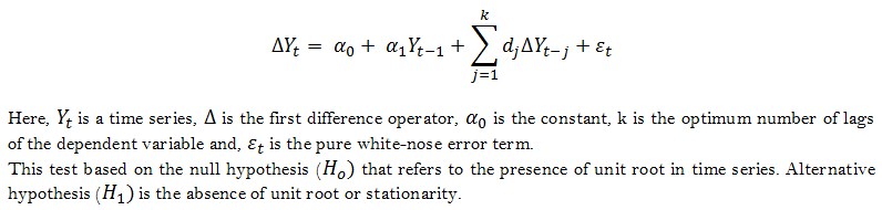
Even though both ADF and PP have little difference, conducting PP with the ADF gives more strong evidence about the presence of stationarity in time series. Statisticians Pierre Perron and C.B. Phillips developed this test by 1988. Both the study has some difference in managing the serial correlation and it is the basic difference of them. PP is a non-parametric test that does not require selecting the level of serial correlation. PP is more effective in longer time series even better than ADF. This test contains significant benefits if there is the presence of moving average components in the time series. Phillips and Perron (1988). Apart from these, PP also holds the type 1 error and sensitivity to structural breaks drawbacks. PP unit root test used by the following equation,
Equation 2 : PP Test
Here, ![]() is the estimated coefficient.
is the estimated coefficient.
This test also based on the null hypothesis ![]() that refers to the presence of unit root in time series.
that refers to the presence of unit root in time series.
Alternative hypothesis ![]() is the absence of unit root or stationarity.
is the absence of unit root or stationarity.
3.5. Kwiatkowski-Phillips-Shin (KPSS) Test
Another unit root test method that examines the presence of stationarity in a time series around a deterministic trend. It conducted based on Ordinary Least square linear regression. This model developed by Denis Kwiatkowski, Peter C.B. Phillips, Peter Schmidt and Yongcheol Shin in 1992. The equation that it follows can derived by three parts,
Equation 3: KPSS Test
Here, ![]() is the random walk,
is the random walk, ![]() is the deterministic trend and
is the deterministic trend and ![]() is a stationary error.
is a stationary error.
Compared to the null hypothesis of the other two tests, KPPS holds the opposite null hypothesis. Presence of stationarity considered as null hypothesis ![]() whereas the absence of stationarity is consider as an alternative hypothesis
whereas the absence of stationarity is consider as an alternative hypothesis ![]() . It is a very important difference because it may happen that time series has no unit root, still be trend stationarity. As it has also a high chance of type 1 error, so it is always, wise to use multiple tests to examine out the presence of unit root in time series which will lead to a more acceptable result.
. It is a very important difference because it may happen that time series has no unit root, still be trend stationarity. As it has also a high chance of type 1 error, so it is always, wise to use multiple tests to examine out the presence of unit root in time series which will lead to a more acceptable result.
3.6. Autoregressive Distributed Lagged (ARDL)
ARDL test used to determine the co-integrating long-run relationship among the variables. It is developed by Peseran and Peseran (1997) and Pesaran, Shin, and Smith (2001) which is used with the unrestricted vector error correction model. This study has used this test in order to find the relationship among financial volatility with other six macroeconomic fundamentals. For finding the co-integrating long-run relationship, different methods are available such as residual bases (Engle & Granger, 1987) test, maximum likelihood-based Johansen and Juselius (1990) and Johansen (1991) tests and some researchers also used Vector Autoregression (VAR) method. However, some drawbacks of all these methods have brought the Ordinary least Square (OLS) based ARDL into the light.
After comparing the ARDL with all other methods, several advantages can be listed such as- First, it doesn’t consider whether the stationarity of the variables has been found either in I(0) or I(1) or combination of both. Second, it is also handy to use with a small sample size consisting of 30 to 80 observations. Third, it can provide simultaneously both long-term and short-run relationships among the variables. Forth, Error Correction Model (ECM) can be derived which refers to the high speed of adjustment of the dependent variable after a short-term shock. Fifth, a structural break issue is not consider by ARDL.
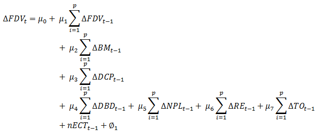
At the very beginning of the whole ARDL test, it is necessary to find whether there is any long-run relationship among the variables or not. If there is any long-run relationship, then long-run estimation for each of the independent variables. So Linear ARDL Bound testing has used to get the evidence of having long run co-integration or relationship among the variables. Considering each of the variables as dependent variable each time, this study has tried to find the best-fitted model for future analysis by formulating the unrestricted error correction model (UECM) which is shown in the matrix form below:
Equation 4: Linear ARDL Bound Test
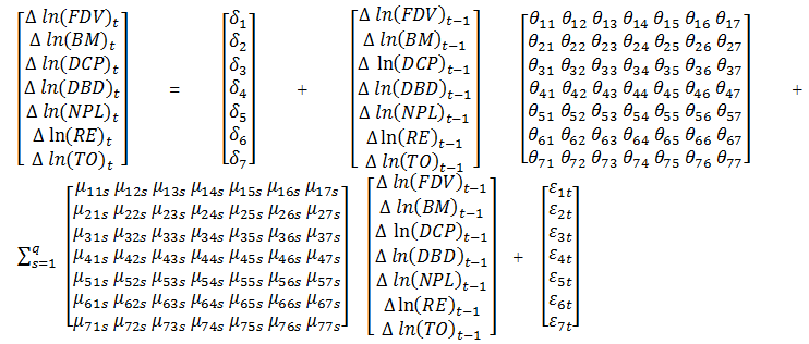
In words,
![]() = There is no long-run relationship among the variables
= There is no long-run relationship among the variables
H_1= There is a long-run relationship among the variables
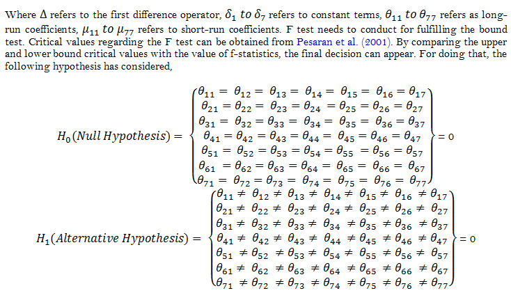
For decision making, whether the null hypothesis will be accepted or not, the following criteria have been proposed by Pesaran et al. (2001). The Summary of decision criteria reported in Table 3.
| Condition | Decision |
| Upper bound of critical value | Rejecting (Confirms Co-integration) |
| Lower bound of critical value | Accepting (Confirms No Co-integration) |
| Upper bound and lower bound of critical value | No Conclusive Decision |
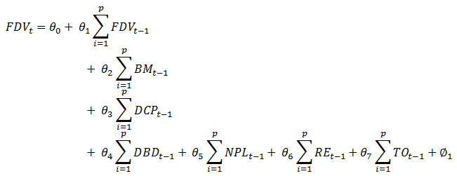
Now, the main ARDL test developed in order to estimate the long-run coefficients separately for each of the independent variables to find the relationship with financial volatility. For doing that, at first, the lag length order of all the variables needs to estimate based on the result of the Schwarz Information Criterion (SIC). In simple terms, lag length refers to the time between the two-time series that are correlate. It is very important to find out which appropriate lag should be included as regressor because considering too many lags as regressor increases the standard error of coefficient estimates, which ultimately leads to forecasting error. While using time series data for the research, Pesaran et al. (2001) suggested that the maximum lag length is 2. The following model has used to estimate the long-run coefficients,
Equation 5 : Long Run Coefficient Test
After finding the evidence of the long-run relationship among financial volatility and the other six variables, now short-run coefficient estimation is possible by formulating the error correction model. In the Error Correction Model, the Error Correction Term refers to the speed of adjustment of the dependent variable to equilibrium after a short-term shock of all the variables. Following model has used to find the short-run coefficients,
Equation 6: Short Run Coefficient Test
4. Empirical Model Estimation and Interpretation
4.1. Unit Root Test Result
The test of unit root for this study conducted by the three most commonly used tests such as Augmented Dickey-Fuller (ADF), Phillip Perron (PP) and Kwiatkowski-Phillips-Shin (KPSS). As all the three tests have few drawbacks, so the combined result will give more verification of the presence of stationarity or non-stationarity.
ADF, which is the updated version of the Dickey-Fuller test, based on the null hypothesis ![]() that refers to the presence of unit root in time series. Alternative hypothesis
that refers to the presence of unit root in time series. Alternative hypothesis ![]() is the absence of unit root or stationarity. By comparing with the significance level 0.05 with the p-value for all the variables at the level and at first difference, we can come to the decision. Table 4 refers that at first level the null hypothesis cannot rejected because p values of all the variables are higher than the 0.05, which also indicates the presence of non-stationarity. However, at first difference, the desired result found, which indicates the presence of stationarity in all the seven variables because of the lower p values than 0.05 significance level.
is the absence of unit root or stationarity. By comparing with the significance level 0.05 with the p-value for all the variables at the level and at first difference, we can come to the decision. Table 4 refers that at first level the null hypothesis cannot rejected because p values of all the variables are higher than the 0.05, which also indicates the presence of non-stationarity. However, at first difference, the desired result found, which indicates the presence of stationarity in all the seven variables because of the lower p values than 0.05 significance level.
The unit root test has also conducted by the PP test considering the same null and alternative hypothesis. Table 4 also provides the same result that has found in the ADF test. All the seven variables exhibit non-stationarity at level, but stationarity at first difference.
The next test is KPSS, which refers to the presence of stationarity as the null hypothesis whereas the absence of stationarity considered as an alternative hypothesis. By comparing critical value at a 5% significance level, which is 0.463000 with the LM statistics value of all the variables, a decision can take. Usually, if LM statistics value is lower than the critical value, then the null hypothesis is accepted which indicates stationarity in time series.
| Variables | Test Name |
||||
ADF |
PP |
KPSS |
|||
t-statistics |
P Value |
t-statistics |
P Value |
LM-S |
|
| BM | 1.841 |
0.999 |
1.841 |
0.999 |
0.753 |
-4.763 |
0.000 |
-4.773 |
0.000 |
0.526 |
|
| dbd | 0.831 |
0.993 |
0.831 |
0.993 |
0.760 |
-4.543 |
0.001 |
-4.524 |
0.001 |
0.280 |
|
| dcp | 2.130 |
0.999 |
1.893 |
0.999 |
0.785 |
-4.821 |
0.000 |
-4.808 |
0.000 |
0.445 |
|
| fdv | -0.920 |
0.771 |
-1.663 |
0.442 |
0.658 |
-12.627 |
0.000 |
-12.642 |
0.000 |
0.500 |
|
| npl | -1.091 |
0.708 |
-0.751 |
0.820 |
0.544 |
-3.880 |
0.006 |
-3.578 |
0.012 |
0.136 |
|
| re | -2.071 |
0.257 |
-1.573 |
0.487 |
0.658 |
-4.377 |
0.001 |
-4.505 |
0.001 |
0.171 |
|
| to | -1.409 |
0.569 |
-1.801 |
0.375 |
0.155 |
-6.045 |
0.000 |
-6.136 |
0.000 |
0.121 |
|
| Note 1: ∆ represents the first difference. Note 2: FDV for financial volatility, BM for broad money, DBD for domestic credit by financial sectors, DCP for domestic credit to private sectors, NPL for non-performing loan, RE for remittance inflow, TO for trade openness. Note 3: ADF for Augmented Dickey-Fuller, PP for Phillip-Perron, KPSS for Kwiatkowski-Phillips-Shin. Note 4: Null hypothesis refers presence of unit root for ADF and PP tests and absence of unit root for KPSS test. |
Now Table 4 indicates LM statistics value is lower than 0.463000 for variable TO only at the level, which indicates stationarity into a variable. However, all the variables except BM and FDV have lower LM statistics value than the critical value at first difference, which indicates acceptance of the null hypothesis. Thus, it refers that even in the order of integration I (1), the KPSS test failed to prove the stationarity in BM and FDV. Similar to ADF and PP, the KPSS test has the chance of providing a type 1 error.
Finally, it is conclude that in a way where ADF and PP tests indicate the stationarity in all the seven variables, but KPSS indicates stationarity only in five variables. Now by considering the fact of the probability of type 1 error in all the three tests, we can conclude the presence of stationarity in the time series of all the seven variables based on the overall results found from these three tests. Lastly, it can be said that variables under consideration are a mix of an order of integration I (0) and I (1).
4.2. Linear ARDL Bound Test Result
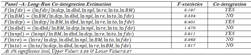
ARDL test prudently used to determine the co-integrating long-run relationship among the financial volatility with the other six macroeconomic factors such as BM, DCP, DBD, NPL, RE, and TO. At the very beginning of the test, it is necessary to find whether there is any long-run relationship among the variables or not by using the Linear ARDL Bound test. If there is any long-run relationship, then long-run estimates are estimate separately for each of the independent variables. By comparing the upper and lower bound critical values with the value of f-statistics, the final decision has taken.
The results in Table 5 refer that, by considering FDV as the dependent variable; there is co-integration among all seven variables because F-statistics value is more than the upper critical bound value at the 5% level of significance, which indicates the rejection of the null hypothesis. Similarly, when DCP and NPL have considered as a dependent variable, there has been co-integration among the variables because of the same ground. However, while considering BM, DBD, RE, and TO as a dependent variables, no evidence has suggested the long-run relationship among these variables.
However, as our main focus of this study is to find the relationship among financial volatility and other six macroeconomic factors, so the result of the linear bound test considering FDV as the dependent variable is our main concern and also it gives almost best-fitted model. Therefore, Linear Bound Test gives us the evidence of having long-run relationship among the variables.
Now, after getting the evidence of having a long-run relationship among the variables, the main ARDL test developed in order to estimate the long-run coefficients separately for each of the independent variables to find the relationship with financial volatility. For doing that, at first lag length order of all the variables has estimated based on the result of the Schwarz Information Criterion (SIC). Table 6 provides the results of lag length criteria based on SIC and selection has done based on the highest value of SIC among the four lags for each of the variables. Results of SIC refers that FDV and RE should be included in this model at first lag. On the other hand, BM; DCP; DBD and NPL should be included in this model at zero lag and the remaining TO should be included in first lag. This lag length selection will guide which coefficient result will be considered.
| Lag | 0 |
1 |
2 |
3 |
Selected Lag |
| FDV | 1.663 |
1.609 |
1.928 |
1.827 |
2 |
| BM | 2.837 |
2.390 |
2.397 |
2.251 |
0 |
| DCP | 2.537 |
1.961 |
1.825 |
1.037 |
0 |
| DBD | 3.408 |
2.974 |
2.963 |
2.682 |
0 |
| NPL | 5.536 |
5.404 |
5.420 |
5.390 |
0 |
| RE | 2.646 |
2.545 |
2.662 |
1.937 |
2 |
| TO | 6.480 |
6.518 |
5.711 |
5.351 |
1 |
4.3. Long Run ARDL Test
After lag selection, estimations for long-run relationships examine and Table 7 (Panel A) shows the results under the ARDL model.
FDV vs. BM: Study findings revealed that broad money has a positive and significant impact on financial volatility in the stock market of Bangladesh. Among all the variables, it has the highest positive contribution in volatility. It also indicates that in the long term, a 100% increase in BM will be the cause of the increase in financial volatility by 13.22% and vice versa. So it can be stated that when the amount of broad money increases in the Bangladesh economy, investors become interested to invest their money by purchasing more stocks which increases immediate price increase of stock for a time being and thus, volatility increases as well. On the other hand, when the money supply decreases in the Bangladesh economy, then people tend to buy fewer new shares. Not purchasing a high amount of new shares within a shorter period decreases the existing volatility. Therefore, it is assume that broad money is a better indicator of volatility in the stock market. This outcome is consistent with the result of Oluseyi (2015); Ndunda et al. (2016); Nikmanesh and Nor (2016); Kumari and Mahakud (2015); Ahmad and Ramzan (2016); Pinjaman and Aralas (2015); Barakat et al. (2016); Nisha (2015); Yadav et al. (2019). On the other hand, this result is inconsistent with Okoro (2017).
FDV vs. DCP: In the long term except for the BM and DBD, the other four independent variables have a negative relationship with financial volatility. Among them, domestic credit to private (percentage of gross domestic product) sector is one of them which has the highest negative contribution to financial volatility. At first lag, the coefficient value is negative 0.139, which indicates a negative and significant relationship with financial volatility. 100% increase or decrease of domestic credit to the private sector cause a 13.9% decrease or increase of financial volatility respectively. It indicates that even if the private sectors like households and businesses get domestic credit easily from financial institutions, they are not willing to invest most of the credit in the stock market; rather they may be interested to invest in other sectors. A slow and less share purchasing tends to decrease existing volatility. Because domestic credit refers mostly to taking a loan from financial sectors. So private sectors do not want to invest this money in a risky stock market like Dhaka and Chittagong stock market. Different market crashes and long-time vulnerability of these two markets lose the confidence of investors. This outcome is consistent with Okech and Mugambi (2016); Okoro (2017) On the other hand, this finding is inconsistent with the findings of Ferreira (2016); Shah et al. (2017).
On the other hand, this result indicates that the decrease in domestic credit increases the stock price volatility. Because, when private sectors do not get a loan, cannot sell the accounts receivables and trade credits, then they face lacking of money and for which, they may start to sell their existing shares, which may lead to decline the stock price immediately, and so, stock volatility increases in Bangladesh market.
FDV vs. DBD: This study finds a positive relationship between DBD and financial volatility, but the impact is not significant as the coefficient value is close to 0.007 only, which also indicates that a 100% increase or decrease in DBD will increase or decrease the financial volatility by 0.7% successively. A similar positive relationship has been found in the study of Banerjee et al. (2019). However, this finding is not consistent with the finding of DCP or it can stated that it provides a contradictory result comparing with DCP. Because of the inclusion of Govt., borrowings from private sectors are the addition in DBD comparing with DCP. Therefore, the relationship between DCP and DBD with financial volatility should be consistent. Nevertheless, here the results indicate a positive or no relationship at all between DBD and volatility. If we look at the probability value at lag o for DBD, it is 0.895, which indicates that it is even not significant at the level of 10%. It also indicates less than a 90% confidence level for this relationship and any result below 80% confidence level is not statistically acceptable. So a conclusive statement about the relationship between FDV and DBD cannot be given from this study, rather a further detailed analysis is required to provide a more in-depth result.
FDV vs. NPL: Non-performing loans (NPL) has also a negative and relatively moderate significant relationship with financial volatility. The coefficient of NPL reveals that a 100% increase or decrease of the non-performing loans in the economy will cause almost a 3% decrease or increase of volatility respectively. This result reveals a clear idea from the perspective of Bangladesh about this relationship. In the last decade, NPL becomes a headache for the Bangladesh economy. It is increasing year by year. Now based on this result, when NPL increases in Bangladesh, it is obvious that financial institutions will have not sufficient amount to give loans or purchase the trade credit; accounts receivables. That means the amount of DCP and DBD go down. Now if the investors do not get sufficient DCP and DBD from FIs, they will not be able to buy new shares. Therefore, a slow and less share purchasing decreases the stock volatility considering all other factors are constant. On the other hand, if in the future, NPL amount starts decreasing in the economy, then people will have more DCP and DBD in their hands. Thus, it may happen that they may start purchasing more shares, which will lead to increased volatility for a time being.
FDV vs. RE: The next variable is RE which has also a negative relationship with financial volatility with a significant one proved by the value of the coefficient of RE. This coefficient value suggests that if there is a 100% increase or decrease happens in RE, then there will be a 9% decrease or increase in financial volatility respectively. This result is consistent with Issahaku et al. (2017). On the other hand, this result is inconsistent with the study of Al Oshaibat (2016); Njoroge (2015); Raza, Jawaid, Afshan, and Abd Karim (2015) (Al Oshaibat, 2016; Njoroge, 2015; Raza, Jawaid, Afshan, & Karim, 2015) . In the last decade, remittance inflow was increasing year by year. This negative relationship indicates that the people of Bangladesh are not willing to invest this remittance amount in-stock purchase although the opposite scenario was expected. It is appear that the Bangladesh stock market has been showing vulnerability for the last decade along with a big crash, which let the investor lose confidence in the stock market. Therefore, they are not willing to take risks with the remittance amount. Consequently, a less purchase of stock reduces the volatility when remittance increases. One further clarification can draw based on the result of coefficient and probability. For the coefficient value of -0.09, the probability value is 0.139, which indicates slightly less than a 90% confidence level about this result, but within an 80% confidence level.
FDV vs. TO: Last one is TO which also provides a negative impact on financial stability or volatility, but not a significant one. Actually, the coefficient value of 0.002 indicates there is almost no relationship between volatility and TO. Nevertheless, the result indicates that if there is a 100% increase or decrease happens in TO, then financial volatility will decreased or increased by only 0.2%, which is very insignificant. This result is consistent with the study of Abubaker (2015); Nikmanesh (2016); Papadamou et al. (2017); Yadav et al. (2019). In the last 6 years, total trade to GDP ratio has been increasing in Bangladesh, which indicates growth in trade. This result indicates that businesses are not willing to invest their excess earning from trade-in purchasing the stock; rather they may invest in other sectors or reinvest. Therefore, change in volatility due to an increase in trade openness is very insignificant.
So from the long run estimation of the coefficient of the variables, it has been found that BM is a better leading positive indicator for financial volatility whereas DCP and RE are two better leading negative indicators of financial volatility.
After finding the evidence of the long-run relationship among financial volatility and the other six variables, now short-run coefficient estimation is possible. Table 7 (Panel B) gives the result of those findings.
FDV vs. BM: The results indicate that broad money has a positive and strong influence on financial volatility in the short run. Compared to the long-run result, there is a stronger relationship between these two because of the higher coefficient value. The coefficient value of BM is 0.185, which indicates that if it is increased or decreased happens in broad money supply in the economy by 100%, there will be an increase or decrease in financial volatility by 18.5% respectively. This result is consistent with Ahmad and Ramzan (2016); Kumari and Mahakud (2015); Pinjaman and Aralas (2015). It is palpable that the reaction of investors will be very quick in case of increased broad money and so, in the short term, this result suggests a stronger relationship than the long term.
FDV vs. DCP: Similar to the long-run relationships, except BM and DBD, the other four variables have a negative impact on financial volatility in the short run too. Among them, DCP is the highest negative contributor on FDV because its coefficient value is 0.1943, which indicates that a 100% increase or decrease in domestic credit in the private sector can cause the decrease or increase of FDV by almost 19.43% respectively. This variable gives a stronger relationship in the short-run compared to the long run. This finding is consistent with Okech and Mugambi (2016); Okoro (2017). However, the opposite result has been found from different studies like (Banerjee et al., 2019; Feng et al., 2017; Ferreira, 2016; Zhou et al., 2015) .
FDV vs. DBD: Again, DBD has a positive impact on financial volatility, but not a significant one similar to long-run relationships. If there is a 100% increase or decrease happens in DBD then financial volatility will increased or decreased by only 0.95% respectively. Again, the relationship between DBD and FDB is inconsistent with the relationship between DCP and FDV in the short run. The same explanation can draw here too.
FDV vs. NPL: The next variable is non-performing loans (NPL) which have a negative impact on FDV with relatively moderate significance. Increasing or decreasing by 100% of NPL causes 4.18% decrease or increase in FDV respectively. In spite of having low significance, it provides better significance in the short-run compared to the long run.
FDV vs. RE: Similar to the long-run relationship, there is a negative and strong relationship between RE and FDV. Actually, there is a stronger relationship exists in the short-run compared to the long run. The coefficient value of RE by 0.146 indicates that if there is a 100% increase or decrease happens in re, then there will be a 14.6% decrease and increase in FDV respectively which is not consistent with Al Oshaibat (2016); Romero (2017).
FDV vs. TO: At last, variable TO also a negative impact on FDV, but with a low significance relationship. Because a 100% increase or decrease in TO will cause only 0.23% decrease or increase in FDV respectively. It indicates a poor impact on stock price volatility.
So from the short run estimation of the coefficient of the variables, it has been found that BM is a better leading positive indicator for financial volatility whereas DCP and RE are two better leading negative indicators of financial volatility. Compared to long-run co-integration, these variables provide a stronger impact on FDV in the short run. This study provides results of both short and long run in a similar direction and a similar explanation can presented for the short run just like the long run. Just because of the quick reaction after a change in any of these variables, this study provides a stronger relationship in the short run compared to the long run.
After conducting this co-integration test by using the ARDL model, a Vector Error Correction test has conducted in order to find the short-run dynamics of the long-run equilibrium relationship. In other words, it estimates both short term and long-term effects of two-time series on another. Considering lag 1 as the standard one, the value of error Correction Term (ECT) is a negative and significant one as it is more than negative 1 (-1.38). This refers that financial volatility has a co-integrating relationship with all independent variables. It also refers that there is a high speed of adjustment of the dependent variable to equilibrium after a short-term shock of all the variables.
For the OLS test, lag 1 has considered as a standard one and this lag 1 will considered as the foundation of all the results of these OLS tests except for one test.
At first, refers to the coefficient of correlation that measures the strength of the linear relationship between two variables. On the other hand, adjusted is suitable in the case of multiple independent variables. As this study includes six independent variables, so this study is focused on adjusting Table 7 (Panel C) provides that value of adjusted is to 0.854, which refers that financial volatility, can be explained by 0.854 or 85.4% by all six independent variables. In other words, these six independent variables are 85.4% responsible for the changes in financial volatility. Firm-specific factors or other reasons are 14.6% responsible for the change of FDV.
The standard error of regression refers to the average error of the regression model or how inaccurate the estimates. The smaller value of standard error indicates that data are close to the regression line and regression analysis can used to predict the dependent variable with very little error. In this study, a very small standard error of regression found equal to 0.405, which indicates that OLS capable to predict the dependent variable considering all the independent variables.
F squared statistics measures the effect size that refers to the strength between two variables especially for using the multiple regression analysis methods. This study has evaluated the Cohen’s statistics which refers to that if the value of is more than 0.35, and then there is a large effect size between two variables. In this study, the value of statistics is almost 23.047 which is undoubtedly larger than 0.35. Therefore, it suggests that there is a strong relationship between the dependent and all independent variables separately.
Autocorrelation or serial correlation refers to the correlation of a variable with itself with subsequent observations. The presence of serial correlation in multiple regression is a serious issue for perfect estimation. Because the error of one observation of a given time period is shifted to the next observation considering the future time. So determining whether the time series has serial correlation or not, is a vital issue for multiple regression analysis. In this study, the value of the serial correlation of this time series is 0.233, which refers that there is a weak positive serial correlation among the different observations of variables. So observations can considered as independent.
One important assumption of OLS regression analysis is that variance of the residual term is constant or almost constant that refers to homoscedastic and having non-constant variance of residual terms refers to heteroskedastic, which creates obstacles for regression analysis to give a good explanation of the performance of the dependent variable. According to the NCV test p-value is the less than the significance level of 0.05, which indicates the absence of heteroscedasticity in this regression model.
The presence of normally distributed data is an important aspect of regression analysis. If the residuals not distributed normally, the result of regression analysis cannot be accurate. Though based on lag 1, the p-value is less than the significance level of 0.05, which indicates the absence of non-normal data; this study can further analyse the normality test based on lag-2 and lag 3 which provide higher p-value than the significance level. So overall, it said that the data of this time series is normally distributed.
RESET test conducted for determining the different types of specification errors such as the absence of any relevant independent variable and incorrect functional form. In this study, it has tried to find out whether any relevant variable has omitted or not and for that, the null hypothesis has made indicating no omitting of any relevant variable. Here, the value of F statistics (0.622) is more than the significance level of 0.05, which indicates the acceptance of the null hypothesis. Therefore, it refers to that; no relevant variable has omitted for conducting this study.
Then, the above analysis based on the seven findings of the OLS study confirms the robustness of the relationship between financial volatility and other independent variables that have found from the test of ARDL.
5. Conclusions
A stable and structured capital market considered as the backbone of an economy. If a country wants continuous growth in the economy, then ensuring the growth of different business organizations is very vital and the growth of those businesses largely depends on the capital raised from the capital market. Because raising capital from the capital market is convenient and cost-effective for businesses. However, if an economy tied up with a vulnerable or volatile capital market, then it becomes very difficult for them to raise a huge amount of capital for continuous growth. However, in the last decade, the economy of Bangladesh was rising; but there was very little contribution from the capital market. High remittance inflow, RMG and agricultural sectors are behind this. However, if Bangladesh wants to achieve its vision of becoming a developed country within 2041, then without a stable and efficient capital structure, it would not be possible at all.
| Panel A: Long-run | ||||||||
| Variables | Regressors (Lag) |
|||||||
0 |
1 |
2 |
3 |
|||||
| BM | 0.132 *[2.005] |
0.140 ** [2.215] |
-0.107** [-1.003] |
-0.347 **[-2.603] |
||||
| DBD | 0.007[0.133] |
-0.013 [-0.253] |
0.141 *[1.873] |
0.232 **[2.325] |
||||
| DCP | -0.139***[-3.156] |
-0.131***[-3.108] |
0.020** [0.295] |
0.177 *[2.214] |
||||
| NPL | -0.030 **[-2.280] |
-0.026**[-2.070] |
-0.071***[-3.462] |
-0.194***[-5.259] |
||||
| RE | -0.021 [-0.452] |
0.010 [0.217] |
-0.090** [-1.550] |
-0.329***[-3.690] |
||||
| TO | -0.002 [-0.351] |
-0.002 [-0.278] |
-0.002 [-0.478] |
-0.026 **[-2.929] |
||||
| Panel B: Short-run | ||||||||
| Variables | Regressors (Lag) |
|||||||
0 |
1 |
2 |
3 |
|||||
-1.398***[-8.688] |
-1.381***[-9.123] |
-1.622***[10.440] |
-2.017***[-11.608] |
|||||
-1.398***[-7.587] |
-1.381***[-7.944] |
-1.622***[-8.745] |
-2.017***[-8.199] |
|||||
0.184 *[1.936] |
0.193 **[2.140] |
-0.174 [-1.003] |
-0.670 **[-2.426] |
|||||
0.009 [0.133] |
-0.017 [-0.253] |
0.229 *[1.850] |
0.469 *[2.229] |
|||||
-0.194***[-2.885] |
-0.181***[-2.841] |
0.033 [0.295] |
0.357 *[2.076] |
|||||
-0.041 **[-2.274] |
-0.036 *[-2.052] |
-0.116 ***[-3.287] |
-0.392***[-4.120] |
|||||
-0.029 [-0.453] |
0.014 [0.217] |
-0.146[-1.541] |
-0.661***[-3.262] |
|||||
-0.003 [-0.352] |
-0.002[-0.279) |
-0.005 [-0.478] |
-0.053 [-2.59] |
|||||
| Panel C: Residual Test | ||||||||
| Variables | Regressors (Lag) |
|||||||
0 |
1 |
2 |
3 |
|||||
0.876 |
0.892 |
0.938 |
0.973 |
|||||
| Adjusted | 0.838 |
0.854 |
0.875 |
0.895 |
||||
0.426 |
0.405 |
0.376 |
0.347 |
|||||
22.937 *** |
23.047 *** |
15.031 *** |
12.430 *** |
|||||
0.565 |
0.233 |
11.961 |
16.646 |
|||||
0.277 |
0.231 |
0.247 |
0.740 |
|||||
0.770 |
0.290 |
0.661 |
.191 |
|||||
0.232 |
0.622 |
.889 |
.187 |
|||||
| Note: ***indicates significance at 1% level, ** indicates significance at 5% level, * indicates significance at 10% level. |
Fluctuation in the stock price depends on different types of factors. It can affect by industry or firm-specific factors. It can also affect by both economic and non-economic factors. Which factors and at which level each of the factors affects the financial volatility is very vital to know for all types of investors. Different researchers tried to establish the relationship of different factors with volatility (Asgharian et al., 2015; Haider, 2017; Ibrahim & Alagidede, 2017; Issahaku et al., 2017; Kumari & Mahakud, 2015; Mittnik et al., 2015; Mumo, 2017; Ndunda et al., 2016; Nikmanesh, 2016; Okoro, 2017; Papadamou et al., 2017; Pinjaman & Aralas, 2015) . Different macro fundamental factors affect volatility such as GDP, money supply, CPI, remittance, export-import level, exchange rate, domestic credit, foreign reserve, etc. In this study, six vital macro factors have chosen such as broad money, domestic credit by the private sector, domestic credit to private sectors, non-performing loans, remittance, and trade openness from analysing the context of Bangladesh's economy. The main purpose of this study is to find out which of these six largely affect the volatility in stock price concerning all types of financial institutions of Bangladesh.
Ordinary Least Square Regression analysis based ARDL model has used to reach the purpose of this study. Data has taken from 1976 to 2017 by an empirical study. To conduct any research, it is important to determine whether there exists the presence of unit root in the time series or not. Because the presence of unit root provides unreliable findings. So this study has conducted three popular unit root tests such as ADF, PP, and KPSS and based on the combined results of these three tests, the decision regarding the unit root has been taken which is consistent with studies like (Barakat et al., 2016; Mumo, 2017; Okech & Mugambi, 2016; OlugBenga & Grace, 2015) . Then, Linear ARDL Bound testing has conducted to get the evidence of having a long-run relationship among the variables and to determine, which variable can consider as the best-fitted dependent variable. After that, lag length has been selected for each of the variables and followed by it, the main ARDL test has been done to find the long-run relationship among the volatility and particular variable (Khan et al., 2015; Raza, Jawaid, Afshan, & Abd Karim, 2015). After testing the long-run effect, the short-run study has conducted. This study ends with the residual test (coefficient of determination, standard error, F squared, normality test, RESET test, heteroscedasticity test, and autocorrelation test) which is conducted to support the findings of the ARDL model (Ndunda et al., 2016; Okech & Mugambi, 2016; Raza, Jawaid, Afshan, & Abd Karim, 2015) .
This ARDL test has provided a separate relationship between volatility and one particular variable either a positive or a negative relationship. This study exposes that broad money and stock price volatility has a strong and positive relationship. Changes in broad money strongly affect volatility. Again, domestic credit by financial sectors has a positive influence on volatility, but the relationship is very weak or it can stat that there is no impact of DBD on financial volatility. Now this study finds a negative relationship of volatility with other rest of four variables. Among those four relationships, domestic credit to the private sector and remittance both has a strong relationship. On the other hand, trade openness has a weak relationship with volatility. However, the non-performing loan has a moderate level of influence on stock price volatility. However, this study provides a contradictory result. In general, DCP and DBD should influence the volatility in the same direction. Again, the result of the relationship between DBD and FDV is not supported statistically also. So further research is required to get reliable results about the relationship between DBD and FDV. So finally, a conclusive statement can state that broad money has the strongest influence on the volatility among these six macro fundamental factors.References
Abubaker, R. (2015). The asymmetric impact of trade openness on output volatility. Empirical Economics, 49(3), 881-887. Available at: https://doi.org/10.1007/s00181-014-0899-2.
Afroze, R. (2013). Impact of Mmonetary policy of Bangladesh bank on the performance of stock Mmarket in Bangladesh. ASA University Review, 7(1), 12-26.
Ahmad, N., & Ramzan, M. (2016). Stock market volatility and macroeconomic factor volatility. International Journal of Research, 3(7), 37-44.
Al Oshaibat, S. (2016). The relationship between stock returns and each of inflation, interest rates, share liquidity and remittances of workers in the Amman stock exchange. The Journal of Internet Banking and Commerce, 21(2), 1-18.
Arif, Z. I. (2018). Capital market outlook for 2018. Dhaka Tribune. Bangladesh: The Daily Star.
Arouri, M., Estay, C., Rault, C., & Roubaud, D. (2016). Economic policy uncertainty and stock markets: Long-run evidence from the US. Finance Research Letters, 18, 136-141. Available at: https://doi.org/10.1016/j.frl.2016.04.011.
Asgharian, H., Christiansen, C., & Hou, A. J. (2015). Macro-finance determinants of the long-run stock–bond correlation: The DCC-MIDAS specification. Journal of Financial Econometrics, 14(3), 617-642. Available at: https://doi.org/10.1093/jjfinec/nbv025.
Baharumshah, A. Z., & Soon, S.-V. (2014). Inflation, inflation uncertainty and output growth: What does the data say for Malaysia? Journal of Economic Studies, 41(3), 370-386. Available at: https://doi.org/10.1108/jes-05-2012-0073.
Banerjee, A. K., Pradhan, Tripathy, & Kanagaraj. (2019). Macroeconomic news surprises, volume and volatility relationship in index futures market. Applied Economics, 52(3), 275-287.
Barakat, M. R., Elgazzar, S. H., & Hanafy, K. M. (2016). Impact of macroeconomic variables on stock markets: Evidence from emerging markets. International Journal of Economics and Finance, 8(1), 195-207. Available at: https://doi.org/10.5539/ijef.v8n1p195.
BBS. (2017). National accounts statistics. Banladesh: Bangladedh Bureau of Statistics.
Cai, W., Chen, J., Hong, J., & Jiang, F. (2017). Forecasting Chinese stock market volatility with economic variables. Emerging Markets Finance and Trade, 53(3), 521-533.
Engle, R. F., & Granger, C. W. (1987). Co-integration and error correction: Representation, estimation, and testing. Econometrica: Journal of the Econometric Society, 55(2), 251-276.
Feng, L., Lin, C.-Y., & Wang, C. (2017). Do capital flows matter to stock and house prices? Evidence from china. Emerging Markets Finance and Trade, 53(10), 2215-2232. Available at: https://doi.org/10.1080/1540496x.2016.1180283.
Ferreira, R. T. (2016). Financial volatility and its economic effects. Working papers, Federal Rserve Board. Available at SSRN 3135452.
Galí, J., & Gambetti, L. (2015). The effects of monetary policy on stock market bubbles: Some evidence. American Economic Journal: Macroeconomics, 7(1), 233-257. Available at: https://doi.org/10.1257/mac.20140003.
Haider, S. K. A. (2017). Systematic risk factors and stock return volatility. APSTRACT: Applied Studies in Agribusiness and Commerce, 11(1033-2017-2927), 61-70.
Ibrahim, M., & Alagidede, P. (2017). Financial sector development, economic volatility and shocks in sub-Saharan Africa. Physica A: Statistical Mechanics and its Applications, 484, 66-81. Available at: https://doi.org/10.1016/j.physa.2017.04.142.
Ilahi, I., Ali, M., & Jamil, R. A. (2015). Impact of macroeconomic variables on stock market returns: A case of Karachi stock exchange. Available at SSRN 2583401.
IMF. (2017). World economic outlook database: International Monetary fund.
Issahaku, H., Abor, J. Y., & Harvey, S. K. (2017). Remittances, banks and stock markets: Panel evidence from developing countries. Research in iInternational Business and Finance, 42, 1413-1427. Available at: https://doi.org/10.1016/j.ribaf.2017.07.080.
Johansen, S., & Juselius, K. (1990). Maximum likelihood estimation and inference on cointegration—with appucations to the demand for money. Oxford Bulletin of Economics and Statistics, 52(2), 169-210. Available at: https://doi.org/10.1111/j.1468-0084.1990.mp52002003.x.
Johansen, S. (1991). Estimation and hypothesis testing of cointegration vectors in Gaussian vector autoregressive models. Econometrica: Journal of the Econometric Society, 59(6), 1551-1580.
Kanas, A., & Karkalakos, S. (2017). Equity flows, stock returns and exchange rates. International Journal of Finance & Economics, 22(2), 159-168. Available at: https://doi.org/10.1002/ijfe.1574.
Khan, M. K., Teng, J.-Z., Parviaz, J., & Chaudhary, S. K. (2017). Nexuses between economic factors and stock returns in China. MPRA Paper No. 81017, posted 28 Aug 2017 11:13 UTC. Retrieved from: https://mpra.ub.uni-muenchen.de/81017/.
Khan, M. N., Tantisantiwong, N., Fifield, S. G., & Power, D. M. (2015). The relationship between South Asian stock returns and macroeconomic variables. Applied Economics, 47(13), 1298-1313. Available at: https://doi.org/10.1080/00036846.2014.995360.
Kitatia, E., Zablonb, E., & Maithyac, H. (2015). Effect of macro-economic variables on stock market prices for the companies quoted on the Nairobi Securities Exchange in Kenya. International Journal of Sciences: Basic and Applied Research, 21(2), 235-263.
Kumari, J., & Mahakud, J. (2015). Relationship between conditional volatility of domestic macroeconomic factors and conditional stock market volatility: Some further evidence from India. Asia-Pacific Financial Markets, 22(1), 87-111. Available at: https://doi.org/10.1007/s10690-014-9194-7.
Laichena, K. E., & Obwogi, T. N. (2015). Effects of macroeconomic variables on stock returns in the East African community stock exchange market. International Journal of Education and Research, 3(10), 305-320.
Mittnik, S., Robinzonov, N., & Spindler, M. (2015). Stock market volatility: Identifying major drivers and the nature of their impact. Journal of Banking & Finance, 58, 1-14. Available at: https://doi.org/10.1016/j.jbankfin.2015.04.003.
Mumo, M. P. (2017). Effects of macroeconomic volatility on stock prices in Kenya: A cointegration evidence from the Nairobi Securities Exchange (NSE). International Journal of Economics and Finance, 9(2), 1-14. Available at: https://doi.org/10.5539/ijef.v9n2p1.
Ndunda, A., Kingori, R., & Areimba, J. (2016). Effect of macro-economic factors on the performance of the equity market of Nairobi securities exchange. International Journal of Business and Commerce, 5(9), 22-33.
Nikmanesh, L. (2016). Trade openness and stock market volatility in the ASEAN-5 countries: New evidence using SUR. Investment Analysts Journal, 45(3), 194-211. Available at: https://doi.org/10.1080/10293523.2016.1172806.
Nikmanesh, L., & Nor, A. H. S. M. (2016). Macroeconomic determinants of stock market volatility: An empirical study of Malaysia and Indonesia. Asian Academy of Management Journal, 21(1), 161–180.
Nisha, N. (2015). Impact of macroeconomic variables on stock returns: evidence from Bombay Stock Exchange (BSE). Journal of Investment and Management, 4(5), 162-170. Available at: https://doi.org/10.11648/j.jim.20150405.14.
Njoroge, W. (2015). Effect of diaspora remittance on stock market performance: Evidence from Nairobi Securities Exchange. International Journal of Current Aspects in Finance (IJCAF), 2(2), 1-11.
Okech, T. C., & Mugambi, M. (2016). Effect of macroeconomic variables on stock returns of listed commercial banks in Kenya.
Okoro, C. O. (2017). Macroeconomic factors and stock market performance: Evidence from Nigeria. International Journal of Social Sciences and Humanities Reviews, 7(1), 1-9.
OlugBenga, A. A., & Grace, O. O. (2015). Impact of foreign direct investment on Nigerian capital market development. International Journal of Academic Research in Accounting, Finance and Management Sciences, 5(1), 103-108. Available at: https://doi.org/10.6007/ijarafms/v5-i1/1503.
Oluseyi, A. S. (2015). An empirical investigation of the relationship between stock market prices volatility and macroeconomic variables' volatility in Nigeria. European Journal of Academic Essays, 2(11), 1-12.
Papadamou, S., Sidiropoulos, M., & Spyromitros, E. (2017). Does central bank independence affect stock market volatility? Research in International Business and Finance, 42, 855-864. Available at: https://doi.org/10.1016/j.ribaf.2017.07.021.
Pesaran, M. H., Shin, Y., & Smith, R. J. (2001). Bounds testing approaches to the analysis of level relationships. Journal of Applied Econometrics, 16(3), 289-326. Available at: https://doi.org/10.1002/jae.616.
Peseran, M., & Peseran, B. (1997). Working with microfit 4: Interactive econometric analysis. Oxford: Oxford University Press.
Phillips, P. C., & Perron, P. (1988). Testing for a unit root in time series regression. Biometrika, 75(2), 335-346.
Phiri, A. (2017). Long run equilibrium adjustment between inflation and stock market returns in South Africa: A nonlinear perspective. International Journal of Sustainable Economy, 9(1), 19-33.
Pinjaman, S. B., & Aralas, S. B. (2015). The dynamic stock returns volatility and macroeconomic factors in Malaysia: A sectoral study. South East Asia Journal of Contemporary Business, Economics and Law, 8(3), 33-40.
Raza, S. A., Jawaid, S. T., Afshan, S., & Abd Karim, M. Z. (2015). Is stock market sensitive to foreign capital inflows and economic growth? Journal of Chinese Economic and Foreign Trade Studies, 8(3), 142-164. Available at: https://doi.org/10.1108/jcefts-03-2015-0012.
Raza, S. A., Jawaid, S. T., Afshan, S., & Karim, M. Z. A. (2015). Is stock market sensitive to foreign capital inflows and economic growth? Evidence from Pakistan. Journal of Chinese Economic and Foreign Trade Studies, 8(3), 142-164.
Romero, F. P. (2017). A correlational study between the volatility of the stock returns and remittances, exports, imports and international reserves: Evidence on the Philippine market. Advanced Science Letters, 23(1), 35-39. Available at: https://doi.org/10.1166/asl.2017.7156.
Sakti, M. R. P., & Harun, M. Y. (2015). Relationship between Islamic stock prices and macroeconomic variables: Evidence from Jakarta stock exchange Islamic index. Global Review of Islamic Economics and Business, 1(1), 071-084. Available at: https://doi.org/10.14421/grieb.2013.011-06.
Shah, S. Z., Baharumshah, A. Z., Habibullah, M. S., & Hook, L. S. (2017). The asymmetric effects of real and nominal uncertainty on inflation and output growth: Empirical evidence from Bangladesh. International Journal of Economics and Financial Issues, 7(1), 377-386.
Siddikee, M. N., & Begum, N. N. (2016). Volatility of Dhaka stock exchange. International Journal of Economics and Finance, 8(5), 220-229.
Vo, X. V. (2015). Foreign ownership and stock return volatility–Evidence from Vietnam. Journal of Multinational Financial Management, 30, 101-109. Available at: https://doi.org/10.1016/j.mulfin.2015.03.004.
World Bank. (2019). World development indicators. USA: The World Bank.
Yadav, I. S., Goyari, P., & Mishra, R. K. (2019). Financial integration and macroeconomic volatility: Evidence from Asia. Journal of Economic and Administrative Sciences, 35(2), 94-112. Available at: https://doi.org/10.1108/jeas-12-2017-0118.
Zhou, J., Zhao, H., Belinga, T., & Gahe, Z. S. Y. (2015). Macroeconomic determinants of stock market development in Cameroon. International Journal of Scientific and Research Publications, 5(1), 1-11.