Impact of FDI on Employment Level in Bangladesh: A VECM Approach

Kazi Mohammed Kamal Uddin¹Munem Ahmad Chowdhury^2*

¹Associate Professor, Department of Economics, Comilla University, Cumilla, Bangladesh. ²MSS Student, Department of Economics, Comilla University, Cumilla, Bangladesh.	Abstract This study is designed to investigate the role of Foreign Direct Investment (FDI) in overall job creation in Bangladesh where annual time series data is used spanning from 1991 to 2018. The role of gross domestic products (GDP) and trade openness on employment level are also addressed. Johansen-Juselius cointegration and Vector error correction model are performed to check long run relationship and short run dynamics among the variables. The findings show that there exists co-integrating relations among the variables. Both FDI and GDP have significant positive effect on employment but trade openness possess the negative impact on employment in the long run. But FDI is negatively related with employment in the short run. This paper suggests to concentrate on making efficient policies to attract investors in green field investment which means investing for the establishment of new firms to create job opportunities in a large scale and to give the opportunity and logistic support to the native producers to produce more import substituted goods for reducing import dependence tendency.
Licensed: This work is licensed under a Creative Commons Attribution 4.0 License.
Keywords: Employment FDI Trade openness VECM Cointegration Bangladesh. JEL Classification: F20; C22.
Received: 18 September 2020 Revised: 1 October 2020 Accepted: 12 October 2020 Published: 22 October 2020
( Corresponding Author)*

Funding: This study received no specific financial support.

Competing Interests: The authors declare that they have no competing interests.

1. Introduction

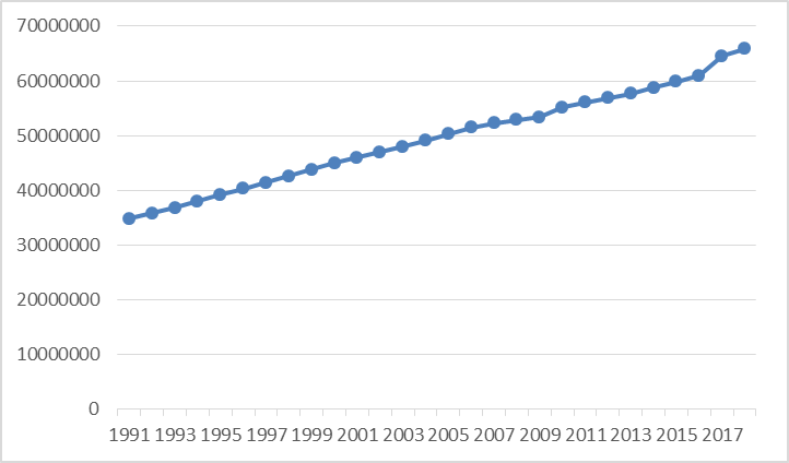
Creating employment opportunities is a great challenge for every developing nation as most of them have a growing population. Employment and economic growth are bound in a circle. When there is an increase in number in employed person in a particular area, then the living standard of people of that area tend to rise. So that their productivity level will also raise. It causes output boom and expansion of that economy. According to Bangladesh Bureau of Statistics (BBS), in Bangladesh in 2016-17 fiscal year, the employment to population ratio was 55.8%.During 2009 in agricultural sector the participation rate of labour was 47.54%. Meanwhile in 2019, it was 39.71% which shows a sharp decline. The reason might be farmers to be down town and their thoughts of stable income. On the other hand both service and industry sector shown a decent rise in it. 35.65% people were engaged in service sector and 16.81% in industry in 2009. In 2019 it becomes 39.76% and 20.53% respectively. A country’s development may not be possible keeping behind its half portion of population. In 2016-17 the total female labour force participation (FLPR) was 36.3% which was so good enough. FLPR in urban area is lower than the rural area.

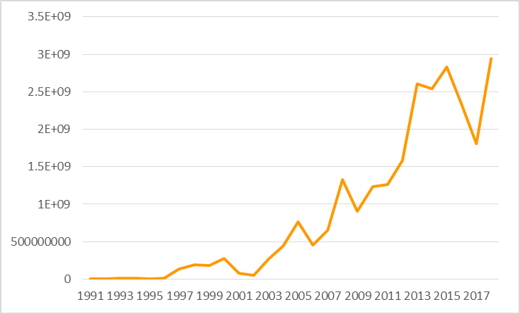
Foreign direct investment (FDI) has been in good shape in recent years. Bangladesh received its highest ever FDI inflow in 2018, 3.61 billion US dollar, according to United Nations Conference on Trade and Development (UNCTAD). The growth rate was around 65%. It becomes the second highest recipient of FDI in South Asia. It was 1.07% of the Gross Domestic Product (GDP). The biggest part of the FDI has been invested in manufacturing sectors over years. Then telecommunication and transportation sectors are the second grossing sector. Till 1990 the amount of FDI wasn’t in a position to be mentioned. After that it has tended to rise but for socio-political instability and lack of adequate business environment the rate of growth was inconsistent. But the recent scenario is quiet pleasant.

For meeting the larger demand of this growing population net trade of goods and services of Bangladesh is still negative. It means total amount of import is greater than export. The total share of import in GDP is 23.44% and export is 14.801%.

The total volume of export of goods and services was 40.558 billion US dollar in 2018 whereas it was 1.867 billion US dollar in 1990 and 18.457 billion US dollar in 2010. Which shows a radical growth. The major export receipts countries are USA, UK and Germany. The largest share of export belongs to readymade garment, mostly 80%. Jute and jute based product, frozen fish, leather, plastic product, petroleum and pharmaceuticals are also some major commodities which are exported. According to Bangladesh bank, exports receipts by EPZ was 6.03 billion USD in 2018-19 fiscal year which was 5.785 billion in 2017-18. As it is known that investment enlarges the size of the firm by improving production facilities and increasing in production of output. So it needs more worker to complete the process. From this the raised question behind this study, does FDI have any impact on the overall employment level in Bangladesh? If it does, then what is the direction of this relationship? Is it positive or negative?

2. Literature Review

Several studies have been done on the relationship of FDI & employment and trade & employment. In 90’s, Vietnam was introduced with FDI boom, but there were no positive effect on employment either directly or indirectly. Jenkins (2006) found that crowding out effect and capital intensive production were main reasons behind this. Recently government of Bangladesh has declared to establish 100 new Export Processing Zone (EPZ), Special Economic Zone (SEZ) and Economic Zone (EZ) in the next 15 years, where it has only 9 EPZ till this day. FDI with EPZ seems to be a powerful engine for job creation in developing countries like Mauritius (Rama, 2003). FDI may induce the economic mobility of such specific area. In Pakistan, India and China, FDI should not be taken as an instrument for employment generation directly. It might have an indirect effect which means it stimulates the economic growth and that would help to create appeal for broadening the labour market (Rizvi & Nishat, 2009). Working on a developing country like Ghana where the level of unemployment is very high, Abor and Harvey (2008) concluded that FDI could be an integral part of their growth as well as generate a large scale employment opportunities. Craigwell (2006) found same conclusion on Caribbean region. By using Granger panel causality test it was found that there was a positive relation between FDI and employment and this was possible for effective trade policy and human capital. Brincikova and Darmo (2014) studied about the V4 countries (Czech Republic, Hungary, Poland & Slovakia) and concluded that there was no significant impact of FDI inflow on unemployment, but GDP growth can be influenced. During the period 1980-2006, in Latin America, FDI have generated employment growth due to their higher productivity and included a significant amount of women employer in several sectors. Which have helped them putting to use the unutilized resources for boosting their growth pace (Vacaflores, 2011). Ernst (2005) have studied the data of 1990s for Argentina, Brazil & Mexico, and found that except Mexico FDI had a negative effect on others. He explained the reason behind that FDI was entered into the market as brownfield investment which means investment in existing firm or industries by merging or acquisition. That things shaded the job creation. A similar reason have been witnessed in Malaysia for having no long run relationship between the employment variable and FDI, using the data span 1990 to 2007 and ARDL bound approach, Pinn et al. (2011). By using Engle-Granger cointegration method Liu (2012) finds that employment in secondary and tertiary industry can be promoted in the long run by growth FDI and there is a bidirectional linkage between FDI and tertiary industry’s employment level. FDI also helps in upgrading the structure of Chinese industry and elevate employment structure towards optimum level. With the increasing volume of trade, firms would like to introduce advance technology regarding the exited amount of labour. It seems like the labour demand curve wouldn’t shift, but the wage level rises for efficient labour forces (Greenaway, Hine, & Wright, 1999). Trade could be harmful for employment growth in developing country like Nigeria, Asaleye, Okodua, Oloni, and Ogunjobi (2017). Higher trade had caused more demand for efficient and skilled labour in Brazil in 80s and 90s to compete with the pace of liberalization, so unemployment might increase as most of the labours were unskilled and poverty also hadn’t been reduced in significant amount that time (Carneiro & Arbache, 2002). Kien and Heo (2009) examined generalized method of moments model for the Vietnam’s liberalization scenario for the time span 1999-2004 and found that export extension creates more labour demand in industrial sector than before because increasing rate of output demands more employee to keep the market share constant. Salem and Zaki (2019) studied trade reform effect of Egypt’s informal and irregular employ side. There openness evacuate the informal (least productive) firms through crowding out process and make room for the formal (productive) firms. So the competitiveness of world economy formulate the requirement for more skilled body and it causes declining in informal employment. Expansion of export with the assistance of FDI have generated more jobs and induced to transfer the surplus labour of other sectors to the manufacturing sector in Chinese economy (Fu & Balasubramanyam, 2005). In the view point of Raihan (2008) trade liberalization is not only the job creating aspects, it also causes job destruction. In export oriented manufacturing industries it shows positive relationship but import substitute industries experience negative depiction. In nineties, reducing in trade barriers Uruguay economy turned into an open one where firms were seen to be improved with more capital intensive technologies. It caused both job creation and destruction. But the net effect was negative meaning that higher job destruction. Two issues that were main reasons behind this; downsizing of firms and union’s intervention, where latter had the more effect on reducing jobs as well as in capital destruction. Along with all this things the total productivity during that time increased at 3 percent annual rate (Casacuberta, Fachola, & gandelman, 2004).

Most of the above studies were done either in developed countries or developing countries. As per our knowledge goes there is no study on the impact of FDI inflow on employment of Bangladesh. That’s why this study has been designed to fill up this gap.

3. Objectives

The main objective of our study is whether there is any relationship between FDI and employment. The specific objectives are;

To detect the way how FDI affects employment.
To determine the impact of trade openness on employment.
To identify the consequences of GDP to the employment.

4. Methodology

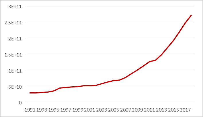
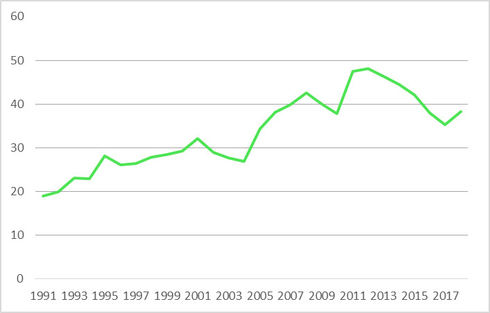
This study used a time series data for 28 years ranging from 1991 to 2018. Employment (EMP) is measured as persons in number and it is collected from International Labor Organization (ILO) database. Gross Domestic Product (GDP) and FDI are measured in current USD and are obtained from world development indicator (WDI) a database of World Bank. Trade openness (TO) is the ratio of sum of total export and total import to GDP and it is obtained from WDI. Since the main objective of this study is to see the impact of FDI on EMP. Hence, in our econometric model EMP is the dependent variable and FDI is the independent variable. To see the impact of GDP and TO, we have used these two variables as independent variables in the model. And their functional relationship is;

As variables are measured in different units, for simplicity of empirical determination, variables have been taken in their logarithmic form to find out their elasticity. We can represent this relationship by the simple OLS regression model as below:

We know that for time series data if we run simple OLS model then it will give us a spurious result. As a result appropriate time series analysis have to be determined for our seeking relationship. To apply the appropriate regression model, it is required to check the stationarity level of all the variables. It means in which level our variables have no unit roots. If our variable is stationary at level then it is regarded as I(0) and if it is stationary at 1st difference, then it is regarded as I(1). Augmented Dickey and Fuller (1979) and Phillips and Perron (1988) test are quite popular approach to do it. The null hypothesis of unit root test is that there is an existence of unit root in a series or the series is nonstationary.

Whenever the time series is stationary, then we need to check whether the variables are cointegrated or not that means whether the variables have long run relationship or not. If the variables are integrated at first difference, I(1), then Johansen and Juselius (1990) causality approach can be performed. For this an unrestricted vector auto regressive (VAR) model can be applied;

Where Z is the matrix of all endogenous variables, P is the lag order and μ is the stochastic error term. Equation 3 can be regenerated in this way;

Where △ is difference operator, Г and Π are the matrices of coefficients and P is lag order which is selected by AIC. Π is the matrix of our all variables and it also indicates long run relationship among variables. There are two test statistics to make it happen; trace statistics & maximum Eigen value. So between two we will go for the first one.

Here r represents the rank of cointegration and the null hypothesis for this equation is there is no co-integrating relationship, r=0.

Once we find our variables are co-integrated then VECM, which is a restricted VAR, is needed to observe the short run dynamics as the long run relationship is confirmed. It also gives both short run and long run relationship’s direction;

Where ect represents the error correction term which tells at what speed our co-integrating equation converges to the equilibrium and also confirms the short run causality of the study variables. φ is it’s coefficient. It should be negative in value and statistically significant.

5. Result and Discussion

Table-1. Unit root test.

	ADF test		Phillips-Perron test		Result
Variable name	At level (t-statistics)	At First difference (t-statistics)	At level (t-statistics)	At First difference (t-statistics)	I(0) or I(1)
LnEMP	-1.442963	-4.497342*	-1.442963	-4.491061*	I(1)
LnGDP	2.435822	-3.328544*	2.146967	-3.264918*	I(1)
LnFDI	-2.075356	-4.675839*	-2.691243	-6.350736*	I(1)
LnTO	-2.106907	-4.893797*	-2.113474	-4.892265*	I(1)

The outcome from the unit root test is reported in Table 1. P-P test is similar to ADF test. Its’ advantage is the robustness with unspecified autocorrelation and heteroscedasticity in the equation. The null hypothesis is that the variable has a unit root. Lag length of our estimation is selected automatically by Schwarz information criterion and max lag was 6. Newey-West bandwidth and Barlett-kernal estimation method is automatically selected for P-P test by E-views. ADF and P-P test don’t reject the null hypothesis at level and reject it at first difference which implies that all of our variables are stationary at first order differentiation, I(1). As all of the variables are integrated at same order, I(1), Johansen-Juselius procedure is the better approach to have co-integrating relations. Before performing cointegration test, we have to know the maximum lag length. Among the above-mentioned information criterions we have selected Akaike Information Criterion (AIC) which possess the lowest value shown in Table 2. So our lag length would be 2 where its’ lowest value held.

Table-2. Lag length selection.

Lag	Log L	LR	FPE	AIC	SC	HQ
0	11.02028	NA	6.70e-06	-0.561623	-0.366602	-0.507532
1	138.1886	203.4693*	9.40e-10	-9.455089	-8.479988*	-9.184637
2	157.2377	24.38278	8.25e-10*	-9.699012*	-7.943831	-9.212200*
3	166.9508	9.324667	1.87e-09	-9.196068	-6.660806	-8.492894

Johansen-Juselius test uses p-values which was given by MacKinnon, Haug, and Michelis (1999). It is told earlier that we only use the trace statistics for estimating hypothesis. From Table 3 when r = 0, the trace statistics exceeds the 5% critical value which indicates rejecting null hypothesis meaning that we have rejected null hypothesis of having no co-integrating equation and accepted null hypothesis of r ≤ 0, i.e. there is one co-integrating equation. So the long run relationship have been identified. The further process is to go through the VECM.

Table-3. Johansan cointegration test for Unrestricted Cointegration Rank Test (Trace).

Hypothesized no. of CE(s)	Null hypothesis	Eigen-value	Trace statistics	0.05 Critical value	Prob**
None*	r = 0	0.657276	55.76743	47.85613	0.0076
At most 1	r ≤ 1	0.536008	28.99668	29.79707	0.0616
At most 2	r ≤ 2	0.323326	9.799487	15.49471	0.2965
At most 3	r ≤ 3	0.001413	0.035340	3.841466	0.8508

Note: Trace statistics indicates co-integrating eqn(s) at the 0.05 level.
*denotes rejection of the hypothesis at the 0.05 level.
**MacKinnon et al. (1999) p-values.

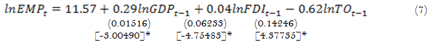
* Significant at 5% level.
** Standard error and t-statistics value are given in first and third braces respectively.

Equation 7 is all about long run relationships. In the long run FDI has a low positive impact on the employment level. We can say it low because 1% increase in FDI will cause 0.04 % increase in employment which may be the causation of capital-based investment. GDP poses a positive and TO has the negative direction. As the country is low-income based, most of her income goes for consumption. In 2018, 31% of GDP was invested. But lack of technical, logistic and infrastructural support, it would not help much. As our import volume is larger than the export one it is obvious to get a negative value. With the expansion of export sector more employment opportunities are created but large-scale import consumption dampen the local productivity. So many employees have been laid off as the sales of local production goes down. It is also revealed from the results that if GDP and trade openness increase by 1%, employment reacts 0.29% and -0.62% respectively. All coefficients are statistically significant at 5%.

Table-4. Co-integrating equations.

Dependent variable: △LnEMP
Variable	Coefficient	Std. Error	t-statistics
ect	-0.11*	0.02165	-5.06499
△LnEMP	-0.51*	0.18518	-2.77725
△LnGDP	0.04	0.02959	1.36353
△LnFDI	-0.005*	0.00190	-3.12419
△LnTO	0.01	0.01555	0.71639
Constant	0.03*	0.00503	6.72657

Note: *indices 5% level of significance.

VECM also shows the short run dynamics of variables and error correction term which is given in Table 4. The coefficient of error correction term is -0.11, it means our short run dynamics converges to the equilibrium at a speed of 11% percent. It is also statistically significant. So there is short run causality. According to the labour force survey of 2016-17, every year about 2 million youths are joining to the labour force. Employment status of previous year has a negative impact. In developing countries number of job seekers are many times more than job opportunities. So when the vacancies are fulfilled in previous year, there is a little chance of creating new spaces at the same amount in present time as there is little scope of capital circulation or investment. FDI impacts on employment is also negative in the short run. Because a larger part of it roaming around capital based investment. The possible reasons may be the investors are more likely to improve the technical system, buying latest technologies, not interested in hiring in more peoples. Rather they hired people more who are more skilled and cut unproductive workers. Merging of companies could be another reason. GDP and trade openness have positive influence but they are not significant so.

Several diagnostic test have been performed which are presented in Table 5 to check the validity of our estimation. By accepting each of their null hypothesis it comes to know that there is no serial correlation and heteroscedasticity in our models. Residuals from the estimated models are normally distributed as the Jarque-bera test fail to reject its’ null.

Table-4. -5. Residual diagnostic tests.

Test	Hypothesis	Test value	Prob.*	Decision
LM	No serial correlation	LM stat- 15.95806	0.4559	No serial correlation
White (cross)	No heteroscedasticity	Chi Sq. – 216.9474	0.1955	No heteroscedasticity
Jarque-Bera	Residuals are normally distributed	JB -4.164020	0.8420	Residuals are normally distributed

6. Conclusion

By applying Johansen cointegration test and VECM we have tried to find out the existence of any kind of relationship between FDI affect the employment level of Bangladesh, using time series data ranging from 1991 to 2018. From our estimated result, FDI have a lower positive impact in employment generation the long run. But have a negative and lower impact in the short run. The larger part of our FDI is not green field investment. Most of it is acquisition or merger of multinational companies or investment in the existing one. In 2018 FDI inflow was $3.16 billion and the $1.5 billion was acquisition of United Dhaka Tobacco by Japan Tobacco. So there is not possible that much of recruiting new members which we forecast just from the total volume. In the long run there may scope for hiring new manpower but our labour force aren’t so skilled enough to meet the total labour demand. As a result a large number of labours are being hired every years from our neighbour countries. Besides when a company meets with more invested capital it is keen to take capital intensive production rather than labours and sometimes may cut its portion for optimal production and cost minimization. So green field invest is a must for creating more jobs in the economy.

For country like ours, developing one, FDI should be more attracted because of lower wage and good macroeconomic stability. But why can’t we attract the foreign investors? There may be numerous number of reason behind this: political instability, lack of adequate infrastructure, favourable tax policy, lack of inducement from government etc. Tax rate should lower for the investor as here one company has to pay 15% tax in its earnings and reserve. Besides the skill of labour forces is a big issue. Our education system doesn’t provide much practical or real world knowledge to the students. That’s why the bookish knowledge doesn’t help them much to meet the requirements of industries. Education system must be formalized in that way where there will exist the path for practicing the acquired knowledge. Vocational education will help much better in this section.
Trade liberalization can play a key role to generate employment opportunities. But as our balance of payment (BOP) is still negative it can’t be happened. Though our export performance help to gain it but import volume drag the rope hard from behind. So the total impact will stand negative as our results says so. Import substitution is highly required. Those goods which can be produced domestically need to impose restriction in their import. So that domestic producer would be beneficial. But in the free trading world this situation can’t be last long. So to make positive BOP export side should get more concentration. Our exports’ market is expanding gradually, the result of export earnings says so. With the increasing rate of export earning, producers are stimulated to raise their production. So this creates more jobs. To keep this continuity we have to maintain quality lest there is a chance of losing market share. There are increasing number of entrepreneurs who can drag their contribution in the track. Having lack of capital impede them. So there might be policies to provide them loans and insurance on easy terms and sometimes government can subsidize in growing sectors. Rules of custom and export processing should be more simplified. Labour intensive exportable goods and services should be more prioritized. As a part of globalization, e-commerce is now easiest way to sell products to distance area. Proper technological support and collaboration with Multinational and international e-commerce companies will open the door for more cash inflow. As we are going to leave the status of Least Developed countries (LDC), we should be more concern about losing the access of Duty free Quota free market.

This study reveals the impact over total employment level. Sector wise employment would give more concrete calculation and specific idea.

References

Abor, J., & Harvey, S. K. (2008). Foreign direct investment and employment: Host country experience. Macroeconomics and Finance in Emerging Market Economies, 1(2), 213-225. Available at: https://doi.org/10.1080/17520840802323224.

Asaleye, A. J., Okodua, H., Oloni, E. F., & Ogunjobi, J. O. (2017). Trade openness and employment: Evidence from Nigeria. Journal of Applied Economic Sciences, 12(4), 1194-1209.

Brincikova, Z., & Darmo, L. (2014). The impact of FDI inflow on employment in V4 countries 92. Cobiss: Mk-Id 95474442, 245.

Carneiro, F., & Arbache, J. (2002). The impacts of trade openness on employment, poverty and inequality: The case of Brazil. Catholic University Working Paper Series No. 09/02. Retrieved from: http://dx.doi.org/10.2139/ssrn.352300 .

Casacuberta, C., Fachola, G., & gandelman, N. É. S. T. O. R. (2004). The impact of trade liberalization on employment, capital, and productivity dynamics: Evidence from the uruguayan manufacturing sector. The Journal of Policy Reform, 7(4), 225-248.

Craigwell, R. (2006). Foreign direct investment and employment in the English and dutch-speaking caribbean. Port of Spain: International Labour Office.

Dickey, D. A., & Fuller, W. A. (1979). Distribution of the estimators for autoregressive time series with a unit root. Journal of the American Statistical Association, 74(366a), 427-431. Available at: https://doi.org/10.2307/2286348.

Ernst, C. (2005). The FDI–employment link in a globalizing world: The case of Argentina, Brazil and Mexico. Employment Strategy Papers, 17, 1-45.

Fu, X., & Balasubramanyam, V. N. (2005). Exports, foreign direct investment and employment: The case of China. World Economy, 28(4), 607-625.

Greenaway, D., Hine, R. C., & Wright, P. (1999). An empirical assessment of the impact of trade on employment in the United Kingdom. European Journal of Political Economy, 15(3), 485-500. Available at: https://doi.org/10.1016/s0176-2680(99)00023-3.

Jenkins, R. (2006). Globalization, FDI and employment in Viet Nam. Transnational Corporations, 15(1), 115-142.

Johansen, S., & Juselius, K. (1990). Maximum likelihood estimation and inference on cointegration—with appucations to the demand for money. Oxford Bulletin of Economics and Statistics, 52(2), 169-210.

Kien, T. N., & Heo, Y. (2009). Impacts of trade liberalization on employment in vietnam: A system generalized method of moments estimation. The Developing Economies, 47(1), 81-103.

Liu, L.-Y. (2012). FDI and employment by industry: A co-integration study. Modern Economy, 3(1), 16-22.

MacKinnon, J. G., Haug, A. A., & Michelis, L. (1999). Numerical distribution functions of likelihood ratio tests for cointegration. Journal of Applied Econometrics, 14(5), 563-577. Available at: https://doi.org/10.1002/(sici)1099-1255(199909/10)14:5<563::aid-jae530>3.0.co;2-r.

Phillips, P. C., & Perron, P. (1988). Testing for a unit root in time series regression. Biometrika, 75(2), 335-346. Available at: https://doi.org/10.1093/biomet/75.2.335.

Pinn, S. L. S., Ching, K. S., Kogid, M., Mulok, D., Mansur, K., & Loganathan, N. (2011). Empirical analysis of employment and foreign direct investment in Malaysia: An ARDL bounds testing approach to cointegration. Advances in Management and Applied Economics, 1(3), 77-91.

Raihan, S. (2008). Trade liberalization and poverty in Bangladesh. Emerging trade issues for policymakers in developing countries in Asia and the Pacific (pp. 153-172). Bangkok: UNESCAP.

Rama, M. (2003). Globalization and workers in developing countries. Policy Research Working Paper 2958, World Bank.

Rizvi, S. Z. A., & Nishat, M. (2009). The impact of foreign direct investment on employment opportunities: Panel data analysis empirical evidence from Pakistan, India and China. The Pakistan Development Review, 48(4), 841-851. Available at: https://doi.org/10.30541/v48i4iipp.841-851.

Salem, M. B., & Zaki, C. (2019). Revisiting the impact of trade openness on informal and irregular employment in egypt. Journal of Economic Integration, 34(3), 465-497.
Vacaflores, D. E. (2011). Was Latin America correct in relying in foreign direct investment to improve employment rates? Applied Econometrics and International Development, 11(2), 101-122.