Impacts of Covid-19 Pandemic and Persistence of Volatility in the Returns of the Brazilian Stock Exchange: An Application of the Markov Regime Switching GARCH (MRS-GARCH) Model
Carlos Alberto Gonçalves da Silva
Visiting Researcher at the Postgraduate Program in Economics Sciences (PPGCE) - State University of Rio de Janeiro (UERJ), Rio de Janeiro, Brazil. |
AbstractThis article provides a quantitative analysis using the Markov Regime Switching GARCH (MRS-GARCH) model with Gaussian distribution, in order to highlight the dynamics presented by Ibovespa during the period from September 2005 to September 2020, in which the subprime crisis occurred and the COVID-19 crisis started. In particular, it used two regimes (regime 1- low volatility and regime 2-high volatility) in the model so that the market parameters (Ibovespa) behave differently during economic crises with the regimes representative. The Ibovespa remained on regime 1 (low volatility) for three periods, totaling 176 months. In regime 2 (high volatility - 2008 and 2020 crises), it remained for about 5 months, that is, 3 months in the 2008 crisis and 2 months in the COVID-19 crisis. In addition, regime 1 is more persistent, that is, the probability of staying on this regime at a later period is approximately 98.27%, and that of switching to regime 2 is 48.25%. In regime 2, the probability of continuing this regime in the period t + 1 is 51.75%, while the probability of changing to regime 1 is 1.73. |
Licensed: |
|
Keywords: JEL Classification |
|
Received: 20 November 2020 |
|
Funding:Author would like to thank the Research Support Foundation of the State of Rio de Janeiro (FAPERJ) for granting the research grant that made this article possible. |
Competing Interests: The author declares that there are no conflicts of interests regarding the publication of this paper. |
Acknowledgement:Author thank the anonymous reviewers for their helpful comments, which have significantly improved the article. Author grateful to the Postgraduate Program in Economic Sciences (PPGCE) of the State University of Rio de Janeiro (UERJ) for participating as a Visiting Researcher in the FINRISK Research Group approved by Depesq-SR2 / CNPq, dedicated to quantitative finance and risk analysis. |
1. Introduction
Many financial time series, for example, stock returns and exchange rates, are well described by stylized facts such as volatility grouping and excess kurtosis. In order to capture these characteristics in the financial data, the autoregressive conditional heteroskedasticity model (ARCH) was introduced by Engle (1982) to deal with conditional variance, that is, that the conditioned variance fits an autoregressive model on the square of errors. Bollerslev (1986) extended the work of Engle (1982) and developed the GARCH (Generalized Autoregressive Conditional Heteroskedasticity) model that incorporates the conditional variance itself, observed in the past, to the ARCH model. The GARCH model, despite capturing the volatility groupings, does not detect the asymmetry of its distribution. Therefore, models were developed that incorporate asymmetry problems. One of the first asymmetric models was EGARCH (Exponential GARCH), proposed by Nelson (1991); Glosten, Jagannathan, and Runkle (1993) and Zakoian (1994) developed the GJR-GARCH and TARCH (Threshold ARCH) model, respectively.
In recent years, several empirical studies have been carried out applied to financial series. Glosten et al. (1993) showed that the influence of negative events on volatility is greater than that of positive events in the American market.
Research on volatility modeling continued through the incorporation of regimes or states in GARCH models, which makes it state dependent. Hamilton (1988) introduced Markov regime change processes to capture the periodic shift from recessions to the business cycle in the United States. Hamilton. and Susmel (1994) and Cai (1994) incorporated this idea into the ARCH model as a way to model volatility with different states. This was later generalized for Gray (1996) Markov Regime Switching GARCH (MRS-GARCH) models. Dueker (1997) used the same approach as Gray (1996) to overcome the infinite path dependency problem and introduced several alternative MRS-GARCH models. Klaassen (2002) modified Gray MRS-GARCH model and showed that its specification presents significant predictive performance of MRS-GARCH models. Haas, Mittnik, and Paolella (2004) proposed a new method different from Gray (1996) approach and affirm that the analytical treatability of their new model allows the derivation of stationary conditions and dynamic properties. Marcucci (2005) main finding is that the predictive performance of MRS-GARCH models is significantly better than simple regime GARCH models over shorter horizons.
2. Literature Review
Mota and Fernandes (2004) compared models of the GARCH family with alternative estimators based on the opening, closing, maximum and minimum prices of the São Paulo Stock Exchange. The results indicated that the alternative estimators are accurate for the GARCH models. The most accurate volatility estimates in the GARCH class come from the EGARCH (2,3)-M model, according to the REQM (root of the mean square error) and EAM (mean absolute error) criteria.
Morais and Portugal (1999) presented models of the GARCH family that capture different effects observed in financial series, such as the agglomeration of variance, the "leverage" effect and the persistence in volatility. This study compares the volatility estimate of the Bovespa index obtained by deterministic and stochastic processes, covering three troubled periods: the Mexico crisis, the Asian crisis and the Russian moratorium. In the selection of deterministic models, despite the high persistence, the GARCH (1,1) model almost always presented the best performance, describes the estimated volatility relatively better when the period used for analysis is stable, whereas the stochastic model performs better in turbulent periods. Therefore, even with high persistence, the Ibovespa series of returns does not present characteristics of an IGARCH model for the deterministic case, nor of non-stationarity for the stochastic case.The results of the study showed that both processes are able to predict volatility.
Costa and Cerreta (1999) examined the influence of events on volatility in Latin American stock markets, using the GJR-GARCH (1,1)-M model. The study uses daily stock market indices and covers a period from January 1995 to December 1998. The results obtained suggest that the influence of negative events is greater than that of positive events in most countries analyzed.
Klaassen (2002) further developed the MRS-GARCH model by distinguishing two regimes with different levels of volatility. This model was tested using three main series of daily exchange rates in US dollars. GARCH effects are allowed within each regime. The resulting Markov regime change GARCH model improves existing variants, for example, making forecasting volatility over several periods ahead a convenient recursive procedure. Empirical analysis demonstrates that the model solves the problem with high single regime GARCH forecasts and that it produces significantly better out-of-sample volatility forecasts.
A Markov regime switching GARCH model based on normal distributions was proposed by Haas et al. (2004). They applied it to three series of exchange rate returns for the volatility forecast and found better volatility forecasts than conventional GARCH models. Marcucci (2005) compared linear and non-linear GARCH models (GARCH, GJR and EGARCH) with the MRS-GARCH modes in the Gaussian, Student's t and GED distributions for errors. The volatility forecasts of the S&P100 index were determined and the empirical results confirmed that the MRS-GARCH models outperformed the standard GARCH models for short-term volatility forecasts.
Liu and Hung (2010) proposed two types of regime change GARCH jump models based on Maheu and McCurdy (2004) autoregressive jump intensity (ARJI) framework to model nonlinearity in return series. The first type is a Markov regime change model that generalizes the GARCH model by distinguishing two regimes with different levels of GARCH jump volatility and intensity, while the second is a threshold GARCH jump model with an exogenous threshold variable. This model was applied to the Japanese YEN-US Dollar exchange rate and to IBM share price and its results, for the sample period, confirmed the better performance of regime change models than the simple GARCH models.
Walid, Chaker, Masood, and Fry (2011) employ a Markov-Switching EGARCH model to verify the dynamic link between stock price volatility and changes in exchange rates for four emerging countries, covering the period 1994–2009. The results highlight two different regimes, both in the conditional average and in the conditional variance of stock returns. The first corresponds to a high average regime and a low variance and the second regime is characterized by a low average and a high variance. In addition, they present strong evidence that the relationship between the stock and foreign exchange markets is dependent on the regime and the stock price volatility responds asymmetrically to events in the foreign exchange market. The results demonstrate that changes in exchange rates have a significant impact on the probability of transition between regimes.
Kaufmann and Scheicher (2006) applied the MRS-ARCH model carried out within the Bayesian structure to describe the daily German stock index (DAX). Gray (1996) used one month US Treasury weekly rates for the period 1970-1994. The author concludes that the MRS-ARCH model outperforms simple one regime models in performance prediction and reduces the persistence in volatility more than Cai (1994) and Hamilton. and Susmel (1994).
Moore and Wang (2007) analyzed the volatility in the stock markets for five new member states of the European Union (EU), the Czech Republic, Hungary, Poland, Slovenia and Slovakia, applying the Markov regime change model, comprising the period 1994-2000. The results reveal a tendency for emerging stock markets to move from the high volatility regime in the previous transition period to the low volatility regime as they move to the EU. The authors showed that joining the EU caused signs of stabilization in the emerging stock markets by a reduction in its volatility.
Lopes and Nunes (2012) consider a Markov regime switching vector autoregression conditional heteroskedastic model with time-varying transition probabilities allowing for shifting correlations. This model is used to study the case of the Portuguese escudo and the Spanish peseta during the EMS crisis. The results show that, in a crisis situation, the interest rate differential has different effects on the transition probability from the crisis state to the non-crisis state: a perverse effect for Portugal, and a positive effect for Spain. We also find strong evidence of contagion, mostly from the Spanish peseta to the Portuguese escudo, and to some extent from the Portuguese escudo to the Spanish peseta.
Torres (2020) applies Markov models with regime change (Markov-Switching) with two regimes, GARCH variance and with homogeneous Gaussian or t-Student likelihood functions between regimes. It involves actively managing portfolios on the Buenos Aires Stock Exchange and the Mexican Stock Exchange, covering the weekly period from January 2000 to January 2019. When carrying out simulations, he carried out the following investment strategies for a U.S. dollar based investor: 1) invest in the risk-free asset if the probability of being in the high volatility regime at t + 1 is higher than 50% or 2) invest in the stock index otherwise. The results suggest that using the t-Student MS-GARCH model in active administration has the best performance in Argentina and the MS model with constant variance and Gaussian function in Mexico.
Sansa (2020) investigates the impact of the COVID - 19 pandemic on financial markets, covering the period from March 1, 2020 to March 25, 2020 in China and the USA. The results of the study revealed that there is a significant positive relationship between COVID - 19 confirmed cases and the financial markets (Shanghai Stock Exchange and New York Dow Jones). This means that COVID - 19 had a significant impact on the financial markets in China and the USA, in the analyzed period.
The objective of the present work is to analyze, estimate and predict the volatility of the returns of the São Paulo Stock Exchange (Bovespa) using the MRS-GARCH model (1.1) which determines the probabilities of low or high volatility, its persistence, the probable duration of each of the states (regimes), that is, to check how long a period of high (low) volatility is expected to last or what is the probability that it will go to a state of high volatility when the Bovespa index is in low volatility or vice versa. Thus, the Markov Regime-Switching model allows you to answer these questions.
3. Methodology and Data
3.1. Single-regime GARCH Model
Engle (1982) in his seminal work aimed to estimate the variance of inflation in the United Kingdom, based on information and data from the 1970s. The result of his work showed the existence of conditional variance in this series of returns, projecting later a greatness of works on the ARCH model, hereinafter presented. In his second publication, used ARCH modeling to define the risk of an investment portfolio, assuming that it followed a process of conditional variance. In 2001, in the publication “The use of ARCH / GARCH models in applied econometrics”, Engle (1982) through the ARCH and GARCH models, proved that in several financial time series, the various extensions of these models could be tested and displayed, for example, in asset pricing and portfolio analysis, revalidating and corroborating the application of the ARCH model in finance.
The generalization of the ARCH model was developed by Bollerslev (1986) when he presented the GARCH model. The author proposed the insertion of lag variance in the model, a kind of adaptive instrument, whereas in the original ARCH model, the conditional variance is a function of the sample variances. The model empirical presentation was based on the American inflation rate, and shortly thereafter, the model was widely accepted and used, including by Engle (1982).
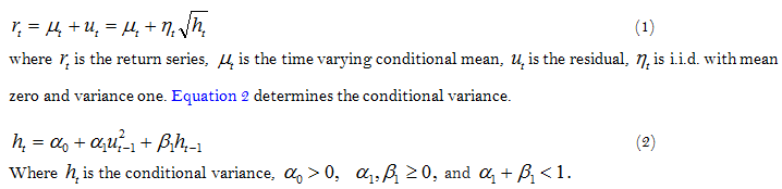
The GARCH (p,q) model proposed by Bollerslev (1986) is a generalization of the ARCH model. The GARCH (1,1) for the series of returns ![]() can be written according to Equation 1.
can be written according to Equation 1.
3.2. Markov Regime-Switching GARCH Model
The Markov Regime-Switching GARCH (MRS-GARCH) model allows the parameters of the conditional volatility to switch across different regimes according to a Markov process thus providing flexibility over the single-regime GARCH models.
This may allow the MRS-GARCH model to capture persistence in conditional volatility in a better way by allowing shocks to have a lower persistence effect during the low volatility regime and more persistent during the high volatility regime. However, a regime switching model is flexible enough to accommodate the volatility clustering, as it can also capture the aftershocks which may take place when large shocks that are not persistent are shadowed by comparatively calm periods.
In a MRS-GARCH (1, 1) model with two regimes, the state variable st evolves according to a Markov chain. More specifically, first-order Markov chain is used in which the probability of the current state also known as transition probability depends only on the most adjacent past state (Gray, 1996). i.e.,![]()
Equation 3 determines the probability of moving from regime i to regime j and ![]() (when
(when![]() ).
).
The transition matrix indicates the probability of switching from state i at time t -1 into state j at t, according to Equation 4.
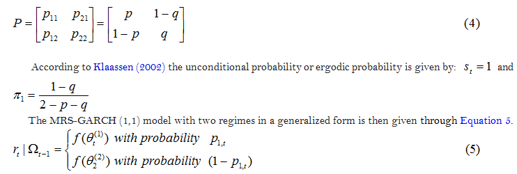
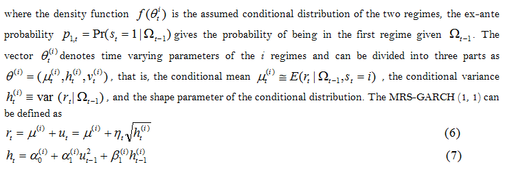
Equation 6 calculates the conditional average of returns from regime i, and Equation 7 calculates the conditional variance of regime i.
Where (i) represents each regime (i=1 or 2). Since the conditional variance ![]() depends on the state dependent
depends on the state dependent ![]() which itself depends on all past states, the estimation of model in (7) is computationally intractable. In order to maximize the likelihood function, all possible unobserved regime paths need to be integrated out which grow exponentially with sample size. One possible by Gray (1996) is to integrate out
which itself depends on all past states, the estimation of model in (7) is computationally intractable. In order to maximize the likelihood function, all possible unobserved regime paths need to be integrated out which grow exponentially with sample size. One possible by Gray (1996) is to integrate out
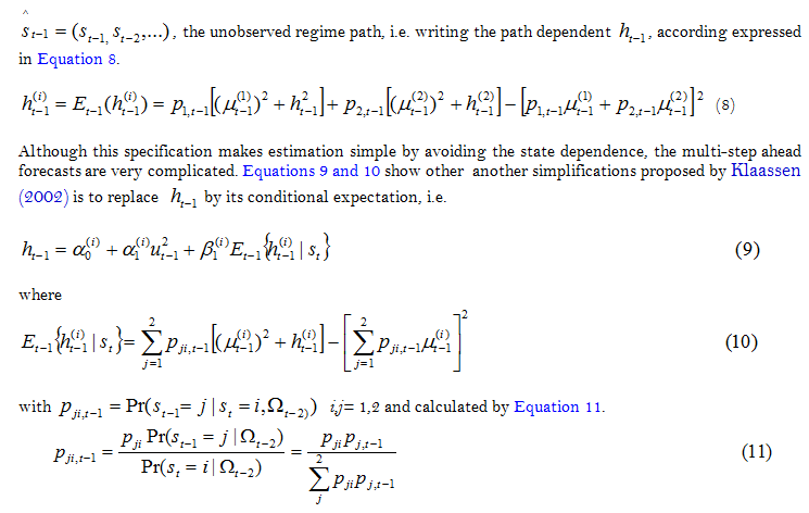
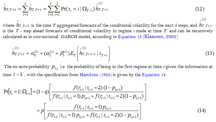
By integrating out the path dependent ![]() , this specification circumvents the path dependence problem similar to Gray (1996) with additional empirical advantage of the efficient use of all available information and theoretical benefit of entailing a simple and easy computation of multistep ahead volatility forecasts ofvolatility. More specifically, the k-step ahead forecasts of volatility at time T can be obtained based on Equation 12.
, this specification circumvents the path dependence problem similar to Gray (1996) with additional empirical advantage of the efficient use of all available information and theoretical benefit of entailing a simple and easy computation of multistep ahead volatility forecasts ofvolatility. More specifically, the k-step ahead forecasts of volatility at time T can be obtained based on Equation 12.
Where p and q are the transition probabilities and f (.) is the density functions in (5).
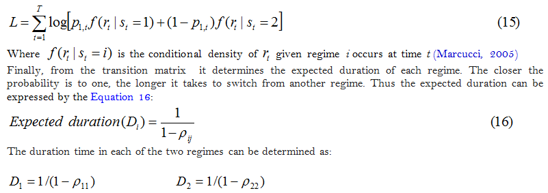
The method of maximum likelihood can be employed to estimate the unknown parameters of the MRS-GARCH (1, 1) model. These parameters can be obtained by maximizing the log likelihood function 15:
3.3. Linearity Test (BDS)
Once it is detected that the distribution is not normal, it is necessary to test the model for linearity. This test was developed by Brock, Dechert, and Scheinkman (1987) used to test if the random variables that compose a series are independent and identically distributed (IID), that is, it can verify several situations in which the variables are not IID, such as non-stationarity, nonlinearity and deterministic chaos. The test is based on the concept of spatial correlation of chaos theory and according to the authors the BDS statistic is formulated through the Equation 17:
3.4. Data
The data used in this study refer to the monthly Bovespa indices, covering the period from September 2005 to September 2020, in a total of 181 monthly observations. The data were obtained from the Yahoo finance website.
4. Empirical Results
4.1 Preliminary Analysis
The daily returns were calculated using the formula: ![]() This
This ![]() represents the number of points at closing on day t and
represents the number of points at closing on day t and ![]() the number of points at closing on the previous day (t-1). Figures 1 and 2 show the behavior of the Ibovespa daily quotation and return series in the period considered.
the number of points at closing on the previous day (t-1). Figures 1 and 2 show the behavior of the Ibovespa daily quotation and return series in the period considered.
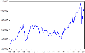
Figure-1. Ibovespa monthly quotes (points).
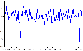
Figure-2. Ibovespa monthly returns.
In the visual inspection of Figure 2, within the analysis period, there is a marked volatility in returns. Thus, it was necessary to test the normality and stationarity of the Ibovespa returns series for application of the MRS-GARCH model.
Some basic descriptive statistics are presented in Table 1. It can be observed that the monthly returns of the Ibovespa present a leptocurtic distribution due to the excess of kurtosis (7,670374) in relation to the normal distribution (3.0), that is, it has heavier tail. It is also verified that the series is negatively asymmetrical which would indicate that stock market lows are more likely than market highs. The analysis of the results shows that both the mean (0.006873) and the median (0.007107) presented values close to zero. The variation between the minimum value (-0,355310) and the maximum value (0.156724) shown by the series can be explained due to some significant oscillations in the index returns. The low value of the standard deviation (0.068466) indicates that, in general, the high variations in the series occurred in a few occasions, that is, in periods of positive and negative peaks. The statistics of Jarque and Bera (1987) indicated the rejection of the normality of the distribution of the series, with p-value equal to zero.
| Statistics | Mean |
Median |
Maximum |
Minimum |
Standard Deviation |
|
| Values | 0.006873 |
0.007107 |
0.156724 |
-0.355310 |
0.068466 |
|
| Statistics | Asymmetry |
Kurtosis |
Jarque-Bera |
p-value |
Observations |
|
| Values | -1.153154 |
7.670374 |
204.6163 |
0.00000 |
181 |
|
The Q-Q Plot represents one of the most used graphic methods to verify the normality of time series. The procedure used consists of graphically comparing the theoretical amounts of the normal distribution with the amounts of the sample data. Figure 3 shows a non-linear relationship between the theoretical and empirical quantiles, which is quite pronounced in the tails of the distributions, indicating heavier tails in the empirical distribution. Therefore, all tests rejected the hypothesis of normality of the analyzed series.
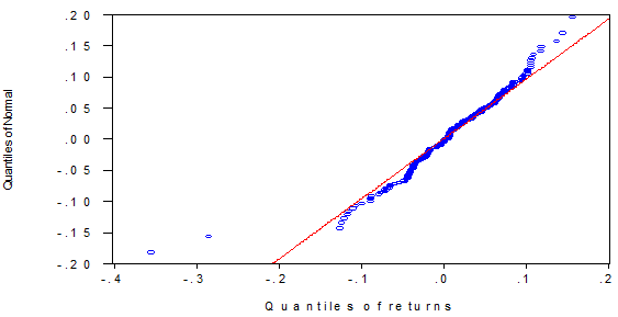
Figure-3. Plot Q-Q of Ibovespa returns.
TheDickey and Fuller (1979); Phillips and Perron (1988); tests and Kwiatkowski, Phillips, Schmidt, and Shin (1992) tests with constant and trend, identified that the Ibovespa return series are stationary and do not contain unitary roots, as presented in the Table 2.
| Variable | ADF |
Critical Value (5%) |
PP |
Critical Value (5%) |
KPSS |
Critical Value (5%) |
| Ibovespa | -11.6044 |
-3.4350 |
-11.5654 |
-3.4350 |
0.0907 |
0.1460 |
Before the estimation of the Markov Regime Switching GARCH (MRS-GARCH) model, a nonlinearity test may be necessary to describe the characteristics of the historical series of the Ibovespa returns. Thus, in T able 3 shows that the results presented indicate the nonlinearity effect, that is, that the probabilities are less than 5% at the significance level, implying a rejection of the null hypothesis that the returns series is linearly dependent.
Dimension |
BDS Statistics |
Statistics Z |
Probability |
2 |
0.0129 |
2.6471 |
0.0081 |
3 |
0.0213 |
2.7485 |
0.0060 |
4 |
0.0229 |
2.4831 |
0.0130 |
5 |
0.0245 |
2.5433 |
0.0110 |
6 |
0.0236 |
2.5466 |
0.0109 |
4.2. Single-regime GARCH
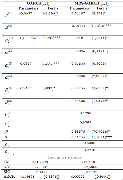
Analyzing Table 4, it can be seen in the simple regime GARCH (1,1) model that the estimated coefficients are statistically significant. The sum of the coefficients was 0.7819, indicating that a shock in the Ibovespa series of returns will have a long-term effect on the volatility of these returns. The persistence coefficient of volatility of 0.7492 confirms that volatility shocks will be slowly weakened by returns, that is, the conditional volatility of Ibovespa returns tend to slowly revert to the average.
In addition, the coefficients ![]() (conditional average),
(conditional average),![]() (constant),
(constant), ![]() (ARCH term),
(ARCH term), ![]() (GARCH term) e are significant for Ibovespa return indexes. The meaning of these parameters is an indication that the lagged conditional variance and the squared disturbance have an impact on the conditional variance, which means that the volatility news from previous periods explains the current volatility.
(GARCH term) e are significant for Ibovespa return indexes. The meaning of these parameters is an indication that the lagged conditional variance and the squared disturbance have an impact on the conditional variance, which means that the volatility news from previous periods explains the current volatility.
4.3. Markov Regime Switching GARCH
In the GARCH model with regime change, the parameters are conditional on the states, which implies that the volatility itself is conditional on the states of low and high volatility. In the GARCH model with regime change, as well as in the traditional GARCH model, volatility depends on past shocks and past volatility.
Table 4 shows the estimates of the MRS-GARCH model (1,1) Gaussian distribuition using the maximum likelihood method, using the OxMetrics 6.0 (PcGive 14) software. The best adjusted model refers to the MRS-GARCH (1.1) in relation to the simple regime GARCH (1.1) model, as verified by the values is log likelihood, is the Akaike (1974) is the Schwarz (1978). In the Markovian regime change model, it was possible to identify a regime with negative returns and high variance (high volatility or low market) and another regime with positive returns and less variance (low volatility or high market). In regime 1 the estimated monthly average return is 1.18% with a variance of 0.1293. Regime 2 identifies a negative average monthly return of 14.7% with a variance of 0.8062.The long-term persistence of Ibovespa volatility, given by the sum, is 0.8096 for regime 1 and 0.9270 for regime 2, which indicates a lesser persistence in volatility in regime 1.
In the matrix of transaction and persistence of the regimes, it appears that the current regime 1 is more persistent, that is, the probability of remaining in this regime in a later period is approximately 98.27%, and that of changing to regime 2 is on the order of 48.25%. In regime 2, the probability of continuing in this regime in the period t + 1 is 51.75%, while the probability of switching to regime 1 is 1.73%. Thus, for the period from September 2005 to September 2020, the expected duration of the current regime 1 is 59 months. In regime 2, the estimated duration is 3 months. The unconditional probability in periods of low volatility is 97.24% and 2.76% in periods of high volatility Table 5.
| Note: *, **, and *** indicate significance at 5%, 1% and 10% respectively. Log is log likelihood, AIC is the Akaike Information Criterion, BIC is the Bayesian Information Criterion |
Transition probability matrix |
Average duration period of regimes |
Regime 1 Regime 2 Regime 1 0.9827 0.0173 Regime 2 0.4825 0.5175 |
Unconditional Duration period probability Regime(1) 0.9724 58.7 Regime(2) 0.0276 2.5 |
Figure 4 shows the behavior of the series of indices, returns, smoothed and predicted probabilities for the Ibovespa state 1 and 2 regimes. The upper panel presents the series of Ibovespa returns, and the middle and lower panels trace the smoothed probabilities for the market in regime 1 (low volatility) and regime 2 (high volatility), respectively.
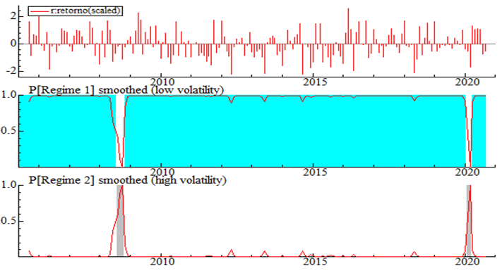
Figure-4. Smoothed probabilities of regimes 1 and 2 obtained from the MRS-GARCH model for Ibovespa returns in the period from September 2005 to September 2020.
From the estimated probabilities, the specific dates of the low volatility (1) and high volatility (2) regimes can be obtained, which are shown in Table 6. The Ibovespa remained under the low volatility regime for three periods, totaling 176 months. In the high volatility regime (crises of 2008 and 2020), Ibovespa remained for about 5 months, that is, 3 months in the crisis of 2008 and 2 months in the crisis of 2020 (period from February 3 to March 31).
Regime 1 (low volatility) |
Regime 2 (high volatility) |
Períod Months Probability |
Períod Months Probability |
2005(9) – 2008(7) 35 0.968 2008(11) - 2020(1) 135 0.990 2020(4) - 2020(9) 6 0.980 |
2008(8) – 2008(10) 3 0.828 2020(2) - 2020(3) 2 0.777 |
In the first period of crisis, beginning in September 2008, there was a significant drop in the Bovespa index, caused by the subprime crisis triggered by the bankruptcy of one of the US investment banks, Lehman Brothers, triggering a crisis in the stock exchanges international standards. After the bank's bankruptcy, the shares started to price an economic crisis, with a strong exit of foreign investors from Brazil. The Ibovespa had a reduction of approximately 60% in 3 months, and it took 14 months for its recovery with the same value before the crisis, after government economic measures.
In the second period of crisis, beginning in January 2020, Ibovespa had a negative impact due to the covid-19 pandemic, which has been generating strong turbulence in world markets and isolation policies to contain the pandemic progress, reflecting on the economy the effects of the shutdown of several economic activities (commerce, industry, aviation and tourism)
The pandemic crisis of the new coronavirus affected the Brazilian economy still fragile, which had not fully recovered from the recession from 2014 to 2016. The historical fall in Brazil PIB in the second quarter with a retraction of 5.5% (negative growth) was pulled by the industry. The sector decreased 12.3% in relation to the first quarter, that is, deepened by the transformation industry, which registered a decrease in the activities of car manufacturers, textile industries and machinery and equipment factories.
5. Conclusion
The objective of the study was to analyze the evolution of Ibovespa returns between September 2005 and September 2020, using the Markov Regime Switching - GARCH model. The best-adjusted model refers to the MRS-GARCH (1.1) in relation to the simple regime model GARCH (1.1), the mean and variance are modified according to the regime (state). Regime 1 (low volatility) expresses an estimated positive average monthly return of 1.18% of Ibovespa returns, with a variance of 0.1293. Regime 2 (high volatility) identifies a negative average monthly return of 14.7% with a variance of 0.8062. The long-term persistence of Ibovespa volatility, given by the sum, is 0.8096 for regime 1 and 0.9270 for regime 2, which indicates less persistence of volatility in regime 1.
In early January 2020, the Ibovespa had a negative impact due to the covid-19 pandemic, which has been generating strong turbulence in world markets and isolation policies to contain the pandemic's progress, reflecting in the economy the effects of the paralysis of several economic activities (commerce, industry, aviation and tourism). Although the downward trend of the stock exchanges is a pattern observed worldwide due to the effects of the covid-19 pandemic, it can justify the sharp percentage of the fall of the Brazilian stock exchange, when compared to other countries, the mass migration of the capital invested in Brazil for US securities and gold, considered safer in times of crisis.
The sharp crisis in the oil sector, which took shape at the beginning of March 2020, caused a drop of 31% in the prices of the commodity in Asian markets. The effects in Brazil can be measured by the devaluation 54,4% of Petrobras preferred stock prices between March 2 and April 1, 2020. In this way, because it has an economy strongly dependent on the export of commodities, among them, oil, and Brazil suffers more significant financial falls than other more developed countries and with less dependence on capital from exports.
The excessive and simultaneous devaluation of Brazilian stocks, reflected in the expressive fall of the Ibovespa, is largely due to pessimistic future expectations, especially in the macroeconomic scenario, as well as the specific situation of each company in its industry affected by the covid-19 pandemic.
In the matrix of transaction and persistence of the regimes, it appears that the current regime 1 is more persistent, that is, the probability of remaining in this regime in a later period is approximately 98.27%, and that of moving to regime 2 is on the order of 48.25%. In regime 2, the probability of continuing this regime in the period t + 1 is 51.75%, while the probability of changing to regime 1 is 1.73%. Thus, for the period from September 2005 to September 2020, the expected duration of the current regime 1 is 59 months. In regime 2, the estimated duration is 3 months.
References
Akaike, H. (1974). A new look at the statistical model identification. IEEE Transactions on Automatic Control, 19(6), 716-723.
Bollerslev, T. (1986). Generalized autoregressive conditional heteroskedasticity. Journal of Econometrics, 31(3), 307-327.
Brock, W. A., Dechert, W. D., & Scheinkman, J. (1987). A test for independence based on the correlation dimension. Department of Economics, University of Wisconsin, SSRI Working Paper, 8702.
Cai, J. (1994). A Markov model of switching-regime ARCH. Journal of Business & Economic Statistics, 12(3), 309-316.
Costa, J. N. C. A., & Cerreta, P. S. (1999). Influence of positive and negative events on the volatility of markets in Latin America. Management Research Notebook, 1(10), 35-41.
Dickey, D. A., & Fuller, W. A. (1979). Distribution of the estimators for autoregressive time series with a unit root. Journal of the American statistical association, 74(366a), 427-431.
Dueker, M. J. (1997). Markov switching in GARCH processes and mean-reverting stock-market volatility. Journal of Business & Economic Statistics, 15(1), 26-34.
Engle, R. F. (1982). Autoregressive conditional heteroscedasticity with estimates of the variances of United Kingdon Inflation. Econometrica, 50(4), 987-1007.
Glosten, L. R., Jagannathan, R., & Runkle, D. E. (1993). On the relation between the expected value and the volatility of the nominal excess return on stocks. The Journal of Finance, 48(5), 1779-1801.
Gray, S. F. (1996). Modeling the conditional distribution of interest rates as a regime-switching process. Journal of Financial Economics, 42(1), 27-62.
Haas, M., Mittnik, S., & Paolella, M. S. (2004). A new approach to Markov-switching GARCH models. Journal of Financial Econometrics, 2(4), 493-530.
Hamilton, J. D. (1988). Rational-expectations econometric analysis of changes in regime: An investigation of the term structure of interest rates. Journal of Economic Dynamics and Control, 12(2-3), 385-423.
Hamilton., J. D., & Susmel, R. (1994). Autoregressive conditional heteroskedasticity and changes in regime. Journal of econometrics, 64(1-2), 307-333.
Jarque, C. M., & Bera, A. K. (1987). A test for normality of observations and regression residuals. International Statistical Review, 55(2), 163-172.
Kaufmann, S., & Scheicher, M. (2006). A switching ARCH model for the German DAX index. Studies in Nonlinear Dynamics & Econometrics, 10(4), 1-37.
Klaassen, F. (2002). Improving GARCH volatility forecasts with regime-switching GARCH. In Advances in Markov-Switching Models. 223-254.
Kwiatkowski, D., Phillips, P. C., Schmidt, P., & Shin, Y. (1992). Testing the null hypothesis of stationarity against the alternative of a unit root. Journal of Econometrics, 54(1-3), 159-178.
Liu, H.-C., & Hung, J.-C. (2010). Forecasting S&P-100 stock index volatility: The role of volatility asymmetry and distributional assumption in GARCH models. Expert Systems with Applications, 37(7), 4928-4934.
Lopes, J. M., & Nunes, L. C. (2012). A Markov regime switching model of crises and contagion: the case of the Iberian countries in the EMS. Journal of Macroeconomics, 34(4), 1141-1153.
Maheu, J. M., & McCurdy, T. H. (2004). News arrival, jump dynamics, and volatility components for individual stock returns. The Journal of Finance, 59(2), 755-793.Available at: https://doi.org/10.1111/j.1540-6261.2004.00648.x.
Marcucci, J. (2005). Forecasting stock market volatility with regime-switching GARCH models. Studies in Nonlinear Dynamics & Econometrics, 9(4), 1558-3708.
Moore, T., & Wang, P. (2007). Volatility in stock returns for new EU member states: Markov regime switching model. International Review of Financial Analysis, 16(3), 282-292.
Morais, I. A. C., & Portugal, M. S. (1999). Modeling and forecasting deterministic and stochastic volatility for the Ibovespa series. Economic Studies, 29(3), 303-341.
Mota, B., & Fernandes, M. (2004). Performance of volatility estimators on the São Paulo Stock Exchange. Revista Brasileira de Economia, 58(3), 429-448.
Nelson, D. B. (1991). Conditional heteroskedasticity in asset returns: A new approach. Econometrica: Journal of the Econometric Society, 59(2), 347-370.
Phillips, P. C., & Perron, P. (1988). Testing for a unit root in time series regression. Biometrika, 75(2), 335-346.
Sansa, N. A. (2020). The impact of the COVID-19 on the financial markets: Evidence from China and USA. Electronic Research Journal of Social Sciences and Humanities, 2, 29-39.
Schwarz, G. (1978). Estimating the dimensional of a model. Annals of Statistics, Hayward, 6(2), 461-464.
Torres, O. V. T. (2020). Investment with Markov-Switching GARCH models: A comparative study between Mexico and Argentina. Accounting and Administration. Next Post, 1-24.
Walid, C., Chaker, A., Masood, O., & Fry, J. (2011). Stock market volatility and exchange rates in emerging countries: A Markov-state switching approach. Emerging Markets Review, 12(3), 272-292.
Zakoian, J.-M. (1994). Threshold heteroskedastic models. Journal of Economic Dynamics and Control, 18(5), 931-955.