Economic Growth and Financial Sector Development: Long-Run Structural Break Cointegration and Short-Run Equilibrium Relationships in the East African Community
Muwanga Sebunya Gertrude
Department of Policy and Development Economics, School of Economics, College of Business and Management, Makerere University, Uganda. |
AbstractThe EAC countries in a bid to boost economic growth (RGDP) and reduce poverty in the region, implemented several financial sector reforms, however, empirical findings have indicated that financial development (FSD) can have a positive, negative or no effect on economic growth. This study investigated this relationship for four EAC countries including Uganda, Kenya, Burundi and Rwanda using individual country Gregory-Hansen-Quandt-Andrews-Muwanga (GHQAM) cointegration procedure based on OLS/ FMOLS estimations. The findings indicate that in the long-run: i). a cointegration relationship exists between financial development and economic growth but it has not been stable for the periods covered; and ii). the elasticity of economic growth to financial development was zero before and after the break for Uganda and Burundi but ranged between 0.000 - 0.3208 and between 0.2178 - 0.3063 for Kenya and Rwanda, respectively, implying an inelastic relationship for all four countries. In the short-run, RGDP did not adjust to changes in FSD in Burundi while 46.36%, 46.3% and 40.67% to 67.47% of the adjustment of the former to changes in the later occurred in the short-run in Rwanda, Uganda and Kenya, respectively. These results signal the need to review and enhance the transmission mechanisms through which financial development affects economic growth and put in place a favourable environment to ensure positive and elastic effects on economic growth. |
Licensed: |
|
Keywords: JEL Classification: |
|
Received: 6 January 2021 |
|
Funding: The paper was funded by School of Economics, College of Business and Management Sciences. |
Competing Interests:The author declares that there are no conflicts of interests regarding the publication of this paper. |
1. Introduction
A solid and well-functioning financial sector plays a significant role in economic development by: promoting economic growth; reducing poverty; assisting the growth of small to medium sized enterprises (SMEs); generating local savings, thus productive investments; facilitating the transfer of international private remittances; among other things. Ultimately, it provides the rudiments of income growth and job creation. Several researchers such as Levine (1997); Abuka and Egesa (2007); Demirgüç-Kunt and Levine (2009) have described the channels through which financial development can lead to economic development through its effects on the intermediate variables. Empirical evidence has also showed that financial sector development is a pre-requisite for economic development, poverty alleviation and economic stability (Beck, 2006; Beck, Levine, & Loayza, 2000; Cihák, Demirgüç-Kunt, Feyen, & Levine, 2013; Levine, 1997; Levine, Loayza, & Beck, 2000; Levine, 2005). This is expected to hold regardless of whether it is defined narrowly or broadly, or basing on the financial system operation environment (which entails establishing robust financial policies and regulatory framework, and improving all the different attributes of the overall environment in which banks operate).
In most developing countries, the emphasis on the private sector as a major engine of growth begun with the IMF and World Bank driven Structural Adjustment Programs (SAPs). Structural reforms played a big role in financial sector development by reducing trade barriers and increasing foreign surplus liquidity in the sector. The resulting increased investment (both local and foreign based) and increased productivity leads to economic development. The mechanism that translates structural reform induced financial development to economic growth is divergent in Africa mainly due to different levels of financial development and liberalization among countries. In Uganda, Kasekende and Atingi-Ego (2003) reported that financial sector reforms and interest rate deregulation appear to have engendered efficiency gains in the banking industry and consequently increasing credit to the private sector is increasing, which turn resulted into economic growth. To-date, the role of the private sector in development is still emphasized by most development agents. Financial sector development is part and parcel of the private sector strategy to stimulate economic growth and reduce poverty.
The EAC member countries in a bid to boost economic growth and reduce poverty in the region implemented several financial sector reforms that can be categorized as either First Generation Reforms (FGR) implemented during the 1990-1998 period or Second Generation Reform (SGR) implemented from 1999 onward. The FGRs included but were not limited to: i). deregulation of the sector whereby the governments reduce their role in the financial sector and allow the market to play a more substantial role in resource allocation by liberalizing interest rates, phasing out subsidies, removal of directed credit, among others; ii). introduction of new prudential frameworks; iii). opening the systems to foreign banks; iv). restructuring and privatizing state owned banks; and v). strengthening supervision and regulation of financial Institutions, for example by strengthening the minimum capital requirements of commercial banks (Abuka & Egesa, 2007; Aleem & Kasekende, 2001; Kasekende & Atingi-Ego, 2003).
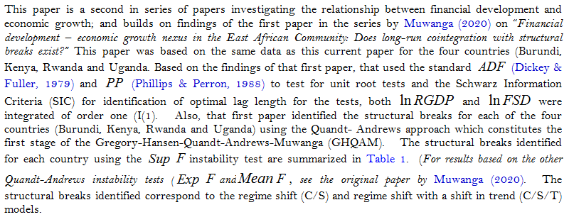
The SGRs were aimed at removing structural obstacles that hinder the financial sectors as they perform their function in the different countries at a national level and the region at large. These reforms focused mainly on the legal, judicial and information infrastructure areas. Abuka and Egesa (2007) review the reforms implemented in the five EAC countries, including Uganda, Tanzania, Kenya, Rwanda and Burundi; (Cihák & Podpiera, 2005) review the financial system structure for Kenya, Tanzania and Uganda; the performance of the banking sector and the role of the banking systems in the face of financial sector reforms; while Egesa (2010) reviews the financial sector reforms in Uganda and the productivity change in the commercial banking sector after the reforms. Muwanga (2020) revealed that structural breaks corresponding to key political events occurred and/or gradual changes which shifted the long-run relationship from one level to another for the four countries, however, that study did not focus on the actual short-run and long-run impact of financial development on economic growth, which is the subject of this paper.
2. Empirical Review
It is expected that financial developments stimulate economic growth and thus reduces poverty, however, empirical evidence reveals that this may or may not be the case (see (Dorosh & Sahn, 2000; Eschenbach, 2004; Esso, 2010b; Fosu, Kimenyi, & Ndung'u, 2003)). Empirical studies on the effect of financial development on economic growth is inconclusive, some indicate no effect, others a positive effect while others indicate a negative effect and yet others indicate no effect. Also, the effects may differ or be similar in the short-run and the long-run.
Studies that have found a positive effect include: Beck et al. (2000); Levine et al. (2000); (Boulika & Trabelisi, 2002); Beck and Levine (2004); Jeanneney, Hua, and Liang (2006); Johannes, Njong, and Cletus (2011); Ngongang (2015); Djoumessi (2009) and Mandiefe (2015) and Kiprop, Kalio, Kibet, and Kiprop (2015). Those who have found a negative effect include Al-Malkawi, Marashdeh, and Abdullah (2012); De Gregorio and Guidotti (1995); Bernard and Austin (2011) amongst others. Lucas (1988) and Stern (1989) on the other hand reported no relationship between financial system development and economic growth. According to Lucas (1988) finance is an “overstressed” determinant of economic growth and concludes that strategies aimed at promoting financial system development wasted resources since they divert attention from more relevant policies such as labour and productivity improvement programs, implementation of pro-investment tax reforms, encouragement of exports; amongst others. Other researchers, (Boulika & Trabelisi, 2002; Güryay, Safakli, & Tüzel, 2007; Islam, Habib, & Khan, 2004; Robinson, 1952) argue for the reverse relationship, whereby financial system development is influenced by economic growth. Their argument is based on the fact that as an economy grows the financial sector responds to the demands of the economy. Otherwise, if it does not, the growth in the economy will be choked as a result of insufficient monetary assets necessary to honour the increased transactions in the economy.
Other researchers have suggested the extreme scenario where financial system development is anti-growth (Buffie, 1984; Van Wijnbergen, 1983) since it facilitates risk amelioration and efficient resource allocation which in turn reduces the rate of savings and risk, consequently leading to lower economic growth (Levine, 2004). Aghion, Howitt, and Mayer-Foulkes (2004) also found an insignificant direct impact of financial development on economic growth, implying zero effect; and further concluded that the level of credits as a percentage of GDP influences growth only in the intermediary stages of development.
Puatwoe and Piabuo (2017) indicated that financial development can have a differing or similar effect in the short-run compared to the long-run; and that the results depend the measures of financial development. They indicated that in Cameroon, financial development measured by monetary mass (M2) and government expenditure had a positive effect while that measured by deposits, private investment had a negative deposits and private investment on economic growth in the short-run; while in the long-run it had a positive and significant impact on economic growth regardless of the measure used.
The above findings reveal divergent views regarding the effect of financial development on economic growth as well as the direction of causality. The divergent views are the consequence of: changing dynamics of financial policies in the countries studied; the response of these economies to policies; the financial sector reforms implemented; varying levels of development, governance and environment in which the financial sector operates, among other factors. Thus, being a pre-requisite for economic growth does not make financial development a necessary and sufficient condition for economic development and poverty alleviation. It is possible to have financial development which is followed by economic decline and/or stagnant growth especially if the transmission channels fail to deliver the desired effects. Since EAC implemented financial reforms with the ultimate aim of achieving economic growth and poverty alleviation, it is necessary to investigate the effects of financial development on economic growth and poverty reduction in all the EAC countries both in the short-run and the long-run. This study addressed this gap by determining whether financial development stimulated or deterred economic growth in the EAC covering the period but not limited to the period during which the FGR and SGR were implemented; and estimated the elasticities of economic growth to financial sector development taking into account structural breaks.
Following the recommendation by Esso (2010b) and the World Bank (1993) the approach adopted examined the finance-growth effects in a country by country basis since the EAC countries differ in their level of financial development which depends on the country specific policies overtime, the level of development and efficiency of the institutions that implement both the country specific policies and those recommended for the region at large. It is expected that the reforms will lead to either gradual changes in the cointegration parameter and/or lead to structural breaks, implying different cointegration relationships before and after the reforms.
3. Methodology
3.1. Standard and Structural Break Models Description
Given the observed data Yt whereby Yt = (Y1t,Y2t), Yt is real – valued and Y2t is an m-vector, two single equation standard models of cointegration with no structural change and four single-equation structural change models can be identified (Gregory & Hansen, 1996a; Muwanga, 2020; Omisakin, Olusegun, Adeniyi, & Oyinlola, 2012). The standard models are presented in Equations 1 and 2 and are based on the assumption that there is no structural break in the cointegration relationship.

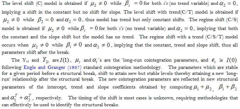
The four structural change models are distinguished based on the assumptions concerning the model specification (with or without a trend variable) and the nature of the shift in the cointegration vector, that is: the level shift (C)- level shift with trend(C/T), regime shift (C/S) and regime shift with a shift in trend (C/S/T). Equation 3 is the general model for structural change models, with the specific models derived from it depending the specific shifts, that is, constant, slope and/or trend shifts which occur, thus the changes of the parameters for the different shifts; and whether the trend variable is included in the model or not (parameter value for the trend variable):

The dependent variable is the logarithm of Real Gross Domestic Product (![]() , and the independent variable is the logarithm of Financial Sector Development (FSD) measured by the ratio of domestic credit to private sector to gross domestic product
, and the independent variable is the logarithm of Financial Sector Development (FSD) measured by the ratio of domestic credit to private sector to gross domestic product ![]() . The measure of the ratio of domestic credit to private sector to gross domestic product ( a credit based measure) was adopted since it is associated with mobilizing savings to facilitating transaction, providing credit to producers and consumers, reducing transaction costs and fulfilling the medium of exchange function of money (Esso, 2010b; Shan & Jianhong, 2006). It also captures the amount of credit channelled by financial intermediaries from savers to the private sector. It can thus be used to measure the effectiveness of the financial sector. Other researchers who have used this measure include (Aghion, Bacchetta, Ranciere, & Rogoff, 2009; Ahlin & Pang, 2008; Beck & Fuchs, 2004; Bolbol, Fatheldin, & Omran, 2005; Emecheta & Ibe, 2014; Honohan, 2004; Kiprop et al., 2015). Other measures such as M2 and M3 have not proved to be good proxies in empirical studies since they reflect the extent of financial services provided by the financial system rather than the ability to channel funds from savers to the private sector. Honohan (2004) who reviewed the pitfalls in using banking depth as a measure of financial development indicated that monetary depth would be a misleading indicator of financial development, particularly if the savings are being mobilized by the state. In the presence of data, indices may represent a better measure of financial development, however, for many developing countries, including those in the EAC, data availability is the major constraint.
. The measure of the ratio of domestic credit to private sector to gross domestic product ( a credit based measure) was adopted since it is associated with mobilizing savings to facilitating transaction, providing credit to producers and consumers, reducing transaction costs and fulfilling the medium of exchange function of money (Esso, 2010b; Shan & Jianhong, 2006). It also captures the amount of credit channelled by financial intermediaries from savers to the private sector. It can thus be used to measure the effectiveness of the financial sector. Other researchers who have used this measure include (Aghion, Bacchetta, Ranciere, & Rogoff, 2009; Ahlin & Pang, 2008; Beck & Fuchs, 2004; Bolbol, Fatheldin, & Omran, 2005; Emecheta & Ibe, 2014; Honohan, 2004; Kiprop et al., 2015). Other measures such as M2 and M3 have not proved to be good proxies in empirical studies since they reflect the extent of financial services provided by the financial system rather than the ability to channel funds from savers to the private sector. Honohan (2004) who reviewed the pitfalls in using banking depth as a measure of financial development indicated that monetary depth would be a misleading indicator of financial development, particularly if the savings are being mobilized by the state. In the presence of data, indices may represent a better measure of financial development, however, for many developing countries, including those in the EAC, data availability is the major constraint.
3.2. Estimation Procedure
The estimation procedure applied in this study involved four stages. The first step involves testing the data series for stationarity; the second step involves identification of structural breaks and testing for cointegration; the third stage involves estimation of the cointegration equation; and the fourth stage involves estimating the ECM if cointegration exists.
3.3. Testing for Unit Roots
This stage involves testing for cointegration using the conventional Augmented Dickey Fuller ![]() (Dickey & Fuller, 1979) and Phillip-Perron (Phillips, 1987; Phillips & Perron, 1988) test statistics to establish whether cointegration exists using the conventional test statistics.
(Dickey & Fuller, 1979) and Phillip-Perron (Phillips, 1987; Phillips & Perron, 1988) test statistics to establish whether cointegration exists using the conventional test statistics.
3.4. Identification of Structural Breaks and Testing for Cointegration
This paper employed a two-step error-correction model (ECM) to investigate the long-run and short-run cointegration relationships, between financial sector development (FSD) and real gross domestic product (RGDP) using the Gregory-Hansen-Quandt-Andrews-Muwanga![]() cointegration approach (Muwanga, 2020). This procedure is similar to the Gregory and Hansen (1996a); Gregory. and Hansen (1996b) threshold cointegration test which explicitly incorporate a break in the cointegration relationship referred to as the Gregory-Hansen-Quandt-Andrews (GHQA) approach and the Fully Modified Ordinary Least Squares (FMOLS) approach.
cointegration approach (Muwanga, 2020). This procedure is similar to the Gregory and Hansen (1996a); Gregory. and Hansen (1996b) threshold cointegration test which explicitly incorporate a break in the cointegration relationship referred to as the Gregory-Hansen-Quandt-Andrews (GHQA) approach and the Fully Modified Ordinary Least Squares (FMOLS) approach.
It involves two-stages. The first stage involved testing for co-integration using the conventional Augmented Dickey Fuller ![]() (Dickey & Fuller, 1979) and Phillip-Perron (Phillips, 1987; Phillips & Perron, 1988) test statistics to establish whether cointegration exists using the conventional test statistics while the second stage, co-integration tests are conducted by allowing structural break(s) established using the Quandt-Andrews procedure (Andrews, 1993; Andrews & Ploberger, 1994; Quandt, 1960) in the long-run
(Dickey & Fuller, 1979) and Phillip-Perron (Phillips, 1987; Phillips & Perron, 1988) test statistics to establish whether cointegration exists using the conventional test statistics while the second stage, co-integration tests are conducted by allowing structural break(s) established using the Quandt-Andrews procedure (Andrews, 1993; Andrews & Ploberger, 1994; Quandt, 1960) in the long-run
equation and testing for co-integration using the Quandt and Andrew instability tests- ![]() and the Mean
and the Mean ![]() tests (Andrews, 1993; Quandt, 1960) and the Hansen L statistic -
tests (Andrews, 1993; Quandt, 1960) and the Hansen L statistic -![]() (Hansen, 1990; Hansen, 1992) as well as standard ADF (Dickey & Fuller, 1979) and/or the
(Hansen, 1990; Hansen, 1992) as well as standard ADF (Dickey & Fuller, 1979) and/or the ![]() (Gregory & Hansen, 1996a). Similarities with the Gregory and Hansen approach lie in fact that this approach incorporates a structural break at an unknown period of time, and estimates the structural break equations using ordinary least squares (OLS) and uses a unit root test determine whether to the regression errors are stationary thereby establishing co-integration if the error terms are stationary (Gregory & Hansen, 1996a). The time break
(Gregory & Hansen, 1996a). Similarities with the Gregory and Hansen approach lie in fact that this approach incorporates a structural break at an unknown period of time, and estimates the structural break equations using ordinary least squares (OLS) and uses a unit root test determine whether to the regression errors are stationary thereby establishing co-integration if the error terms are stationary (Gregory & Hansen, 1996a). The time break ![]() is initially treated as unknown and is determined using the Quandt-Andrews instability tests computed for each break point in the interval [0.15T, 0.85T], where T denotes the sample size. The date of the structural break corresponds to the Supremum
is initially treated as unknown and is determined using the Quandt-Andrews instability tests computed for each break point in the interval [0.15T, 0.85T], where T denotes the sample size. The date of the structural break corresponds to the Supremum![]() , Exponent
, Exponent ![]() and Mean
and Mean ![]() test statistics computed on the trimmed sample.
test statistics computed on the trimmed sample.
Unlike the Gregory and Hansen approach, which uses the smallest values of the standard Augmented-Dickey-Fuller ![]() and Phillip test statistics across all values
and Phillip test statistics across all values ![]() , to test for existence of an endogenously determined structural break and co-integration, the Gregory-Hansen-Quandt-Andrews-Muwanga
, to test for existence of an endogenously determined structural break and co-integration, the Gregory-Hansen-Quandt-Andrews-Muwanga![]() co-integration approach uses i) the instability tests (
co-integration approach uses i) the instability tests (![]() and Mean
and Mean ![]() ) estimated using the FMOLS procedure across all values
) estimated using the FMOLS procedure across all values ![]() to identify the structural break; ii) the OLS procedure to estimate the corresponding OLS cointegration relationship that incorporates the structural break alternative identified; and iii) tests for cointegration either using the standard Augmented-Dickey-Fuller
to identify the structural break; ii) the OLS procedure to estimate the corresponding OLS cointegration relationship that incorporates the structural break alternative identified; and iii) tests for cointegration either using the standard Augmented-Dickey-Fuller ![]() procedure and Phillips test statistics (Phillips, 1987) or by treating the
procedure and Phillips test statistics (Phillips, 1987) or by treating the ![]() statistic obtained for the same equation as the test statistic for the Gregory-Hansen procedure and subjecting it to the Gregory-Hansen critical values. The
statistic obtained for the same equation as the test statistic for the Gregory-Hansen procedure and subjecting it to the Gregory-Hansen critical values. The![]() statistics is used to test the null hypothesis of cointegration with no regime shifts against the alternative of cointegration with a shift in the parameter vector at an unknown point while the
statistics is used to test the null hypothesis of cointegration with no regime shifts against the alternative of cointegration with a shift in the parameter vector at an unknown point while the![]() statisticstest the null of cointegration against the alternative of a random walk type variation in the parameter vector. For a detailed description of the Gregory-Hansen-Quandt-Andrews-Muwanga
statisticstest the null of cointegration against the alternative of a random walk type variation in the parameter vector. For a detailed description of the Gregory-Hansen-Quandt-Andrews-Muwanga![]() cointegration approach, see (Muwanga, 2020).
cointegration approach, see (Muwanga, 2020).
3.5. Estimation of the Long-Run Structural Break Cointegration Relationship
Any of the four structural models can be used to estimate the long-run cointegration relationship. For this study the regime shift (C/S) and regime shift with trend models in Equations 4 and 5 were the candidates since structural breaks corresponding to these models were the ones investigated in the previous stage based on standard models 1 and 2 in Equations 1 and 2, respectively. The regime shift with a shift in trend (C/S/T) is considered to be superior to the models since the other versions of the structural models can be deduced from it, and it has also been and contains a trend which is inherent in most time series.
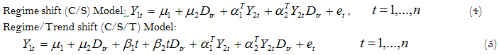
3.6. Estimation of Short-Run Error Correction Model (ECM)
Existence of cointegration based on Quandt- Andrews instability tests, provides the basis for estimating error-correction model![]() in Equation 6.
in Equation 6.
The variables ![]() are as defined earlier. The ECM will be estimated using the FMOLS which does not estimate the short-run elasticity (Tatoglu, 2011) but estimates the speed of adjustment,
are as defined earlier. The ECM will be estimated using the FMOLS which does not estimate the short-run elasticity (Tatoglu, 2011) but estimates the speed of adjustment, ![]() in equation 7, which shows the rate at which the disequilibrium form the equilibrium level is corrected in this current year. The rule for the existence of a short-run equilibrium (Puatwoe & Piabuo, 2017) between financial development and economic growth is that the coefficient of the error correction term should be negative and it should be significant.
in equation 7, which shows the rate at which the disequilibrium form the equilibrium level is corrected in this current year. The rule for the existence of a short-run equilibrium (Puatwoe & Piabuo, 2017) between financial development and economic growth is that the coefficient of the error correction term should be negative and it should be significant.
3.7. Data Sources and Sample Sizes
Financial development (domestic credit to private sector (% GDP)) data was obtained from the World Bank GFDR Report (2016) Report while GDP (GDP constant 2005 US $) data was obtained from the IMF database. The samples varied for the different countries. The same sample size could not be used for all four countries due to data availability constraints. The data periods for the different countries were: 1964-2013 for Burundi, 1961-2013 for Kenya, 1964-2005 for Rwanda and 1982-2013 for Uganda. The data is presented in Appendix Tables 1 and 2.
4. Results
4.1. Stationarity (Unit Root Test) and Structure Break Identification Results
| Country Sample |
Break point Model |
Trimmed Sample |
No. of Breaks compared |
Break Point |
|
| Rwanda (1964-2005) |
Regime shift (C/S) | 1971-1999 |
29 |
1979 |
4.977744 (0.0964)* |
| Regime/ trend shift (C/S/T) | 1971-1999 |
29 |
1994 |
66.922 (0.0000)*** |
|
| Burundi (1964-2013) |
Regime shift (C/S) | 1972-2006 |
35 |
1984 |
34.372 (0.000)*** |
| Regime/ trend shift (C/S/T) | 1972-2006 |
35 |
1995 |
92.09 (0.000)*** |
|
| Uganda (1982-2013) | Regime shift (C/S) | 1987-2009 |
23 |
1988 |
11.830 (0.0002)*** |
| Regime/ trend shift (C/S/T) | 1987-2009 |
23 |
1987 |
23.645 (0.000)*** |
|
| Kenya 1961-2013 | Regime shift (C/S) | 1969-2006 |
38 |
1996 |
103.655 (0.000)*** |
| Regime/ trend shift (C/S/T) | 1969-2006 |
38 |
1972 |
48.7976 (0.000)*** |
| Source: Adapted from Muwanga (2020). Notes: 1Figures in parentheses below test statistics are probabilities, while the ns, *, ** and *** signify lack of significance, significance at 10%, 5% and 1% respectively. 2Probabilities are computed using (Hansen, 1997) method. 3A trimming percentage 15% was used. 4Rejection of the null hypothesis implies presence of cointegration with structural break (or regime shift). 4Both Wald |
The results of the![]() test indicated that at the 1% level of significance, cointegration accompanied by a structural break existed for Kenya, Uganda, and Burundi for both the regime shift and regime shift with trend model. For Rwanda, cointegration existed for both the regime shift with trend model and regime shift level at 1% and 10% levels of significance, respectively. The structural breaks for Model 4 and Model 5 were identified in 1979 and 1994, 1984 and 1995, 1988 and 1987, and 1996 and 1972 for Rwanda, Burundi, Uganda and Kenya, respectively. The structural breaks identified for Model 4 and Model 5 were used to estimate Model 4 and Model 5, respectively using OLS.
test indicated that at the 1% level of significance, cointegration accompanied by a structural break existed for Kenya, Uganda, and Burundi for both the regime shift and regime shift with trend model. For Rwanda, cointegration existed for both the regime shift with trend model and regime shift level at 1% and 10% levels of significance, respectively. The structural breaks for Model 4 and Model 5 were identified in 1979 and 1994, 1984 and 1995, 1988 and 1987, and 1996 and 1972 for Rwanda, Burundi, Uganda and Kenya, respectively. The structural breaks identified for Model 4 and Model 5 were used to estimate Model 4 and Model 5, respectively using OLS.
4.2. OLS Long-Run Cointegration Relationships for Standard and Structural Break Models
Following the results presented above, the regime shift (Equation 4) and regime shift with trend shift models (Equation 5) were estimated for the four countries including Burundi, Kenya, Rwanda and Uganda. In all cases, the residuals from each equation were tested for cointegration using the standard ADF statistic using the standard ADF procedure and the ![]() using the Gregory and Hansen critical values ( as did the first paper in the series). Based on R-2 and the Schwartz and Akaike criteria, the regime shift with trend shift model was better than the regime shift model for all the four countries. Table 2 presents the long run cointegration results for this model for the four countries. (The results for the regime shift model, which are discussed in this paper can be obtained from the author by request).
using the Gregory and Hansen critical values ( as did the first paper in the series). Based on R-2 and the Schwartz and Akaike criteria, the regime shift with trend shift model was better than the regime shift model for all the four countries. Table 2 presents the long run cointegration results for this model for the four countries. (The results for the regime shift model, which are discussed in this paper can be obtained from the author by request).
| Variable | Parameter |
Eq6 Burundi |
Eq6 Kenya |
Eq6 Rwanda |
Eq6 Uganda |
| Sample | 1964-2013 N=50 |
1961-2013 N=53 |
1964-2005 N=42 |
1982-2013 N=32 |
|
| Str. Break point | R |
1995 |
1972 |
1994 |
1987 |
| Constant (C) | µ1 |
19.95 (0.000)*** |
21.435 (0.000)*** |
20.156 (0.000)*** |
21.808 (0.000)*** |
| Str. Dummy (Dtr) | µ2, r |
0.0231 (0.927)ns |
-0.295 (0.4515)NS |
-2.0577 (0.0142)** |
-0.5262 (0.0010)*** |
| Trend (t) | Β |
0.0367 (0.000)*** |
0.0696 (0.000)*** |
0.0226 (0.0033)*** |
0.0043 (0.463)NS |
| (tDtr) | -0.0065 (0.0844)* |
-0.0372 (0.000)*** |
0.0577 (0.0692)* |
0.0536 (0.000)*** |
|
| lnFSD(Y2) | α1T |
-0.0341 (0.3213)ns |
0.0404 (0.7838)NS |
0.2178 (0.0306)** |
-0.0737 (0.5146)NS |
| (Y2Dtr) | α2T |
-0.0873 (0.3838)ns |
0.2804 (0.0737)* |
-0.1242 (0.8512)NS |
0.2051 (0.1385)NS |
| R-2 | 0.965 |
0.997 |
0.833 |
0.998 |
|
| Akaike Inf. | -2.561 |
-3.6433 |
-0.5904 |
-4.464 |
|
| Schw. Crit. | -2.332 |
-3.4203 |
-0.3421 |
-4.189 |
|
| F-statistic | 272.689 (0.000) |
3357.012 (0.000)*** |
41.888 (0.000)*** |
3735.104 |
|
| Res. Unit. Root. Test/Conclusion | -4.952 Cointegration |
-5.6702*** Cointegration |
-4.728*** Cointegration. |
-3.712*** Cointegration. |
The constants parameters were significant in all countries and remained the same before and after the structural break in Burundi and Kenya but declined in Rwanda by -2.0577 after the break in 1994 and in Uganda by -0.5262 after the break in 1987. The trend variable was significant in all the four countries and trend shifts occurred in all four countries. The shifts in Burundi and Kenya were negative while those in Rwanda and Uganda were positive. These results imply that the pace at which economic growth was increasing over time in Burundi and Kenya declined after the structural break but it increased after the breaks in Rwanda and Uganda.
Based on this model it can be concluded that the elasticity of growth to financial sector development was: i). not significantly different from zero (negative and insignificant coefficient of -0.0341 before the break and with an insignificant structural break coefficient of -0.0873) in Burundi before and after the break in 1995 implying no effect financial development on economic growth both before and after the break; ii). not significantly different from zero (positive but insignificant coefficient of 0.0404) before the structural break but was 0.3208 (positive and significant coefficient change of 0.2804 (0.0404 + 0.2804 = 0.3208) after the structural break in 1972 for Kenya, implying no effect of financial development on economic growth before the break but a positive effect after the break (slope shift); iii). 0.2178 for Rwanda before and after the break ((positive and significant coefficient of 0.2178 but insignificant structural break effect of -0.1242) in 1994, implying a positive effect of financial development on economic growth but no slope shift; and iv) not significantly different from zero (negative but insignificant coefficient before the break of -0.0737, and positive and insignificant structural break effect after the break of 0.2051) in Uganda both before and after the break in 1987, implying no effect financial development on economic growth both before and after the break.
These result show that although financial development can have either a positive or negative effect on economic growth. However, since all the negative elasticities (Uganda and Burundi) were not significantly different from zero (see Table 2), it can be concluded that it has had either a zero (Burundi and Uganda) or positive (Rwanda and Kenya) effect on economic development in the four EAC countries. These results indicate that a cointegration relationship exists between RGDP and FSD but it has not been stable for the period under investigation since at least the constant (for Uganda), trend for all countries) and/or the slope (Kenya) parameter has changed over the period. The elasticities (slope coefficients) of RGDP to FSD remained constant (stable) with the exception of that for Kenya which increased from 0.0404 to 0.3208 but is still less than 1 as is the one for Rwanda (0.2178). Those for Uganda and Burundi were not significantly different from Zero. These results signify that after accounting for structural breaks, FSD had an inelastic effect (little or zero effect) on RGDG during the period of study.
4.3. Long-run Fully Modified Ordinary Least Squares (FMOLS) Cointegration Results
Table 3 contains the FMOLS long-run cointegration relationships for the four countries.
Cointegration was established for all countries based on the ADF test whereby, the null of no cointegration was rejected for all countries at the 5% and/or 1% level of significance. These results at the 1% level significance are the same as those obtained for the same model using the![]() test statistic. However, based on the Lc test, cointegration was established only for Uganda at the 10%, 5% and 1% levels of significance since the probability which is greater than 0.2 leads to failure to reject the null of cointegration at all those levels. The other countries, cointegration was established at the 1% level of significance since the null hypothesis of cointegration was rejected at the 5% level of significance for Burundi and Rwanda, and at 10% level of significance for Rwanda but not at 1% level. Considering the 1% level of significance, cointegration was established for all four countries based on the Lc.
test statistic. However, based on the Lc test, cointegration was established only for Uganda at the 10%, 5% and 1% levels of significance since the probability which is greater than 0.2 leads to failure to reject the null of cointegration at all those levels. The other countries, cointegration was established at the 1% level of significance since the null hypothesis of cointegration was rejected at the 5% level of significance for Burundi and Rwanda, and at 10% level of significance for Rwanda but not at 1% level. Considering the 1% level of significance, cointegration was established for all four countries based on the Lc.
| Variable | Parameter |
Burundi |
Rwanda |
Uganda |
Kenya |
| Sample | 1965-2013 N=41 |
1965-2005 N=49 |
1983-2013 N=31 |
1962-2013 N=52 |
|
| Str. Break point | R |
1995 |
1994 |
1987 |
1972 |
| Constant (C) | µ1 |
19.869 (0.000)*** |
20.1378 (0.000)*** |
21.912 (0.000)*** |
21.422 (0.000)*** |
| Str. Dummy (Dtr) | µ2, r |
0.004 (0.9878)ns |
-0.1445 (0.0125)** |
0.0588 (0.000)*** |
-0.3502 (0.4266)ns |
| Trend (t) | Β |
0.0369 (0.000)*** |
0.0139 (0.0672)* |
-0.0022 (0.8334) |
0.0699 (0.000)*** |
| (tDtr) | -0.0065 (0.1042)ns |
0.0564 (0.0816)* |
0.0588 (0.000)*** |
-0.0376 (0.000)*** |
|
| lnFSD(Y2) | α1T |
-0.0523 (0.1539)ns |
0.3063 (0.0056)*** |
-0.1046 (0.5227)ns |
0.0445 (0.7892)ns |
| (Y2Dtr) | α2T |
-0.075 (0.4795)ns |
-0.0156 (0.9815)ns |
0.2493 (0.1759)ns |
0.2977 (0.0919)* |
| R-2 | 0.9605 |
0.8076 |
0.998 |
0.997 |
|
| Long-run variance | 0.0045 |
0.0296 |
0.001 |
0.0017 |
|
| Lc test statistic | 0.8446 (0.0219)** |
0.5812 (0.0710)* |
0.295 (p>0.2) |
0.7381 (0.0332)** |
|
Z- stat |
-32.4376 (0.0129)** |
-29.322 (0.0219)** |
-60.367 (0.000)*** |
-40.4833 (0.0013)*** |
| Notes: Values in parenthesis are probabilities. |
The constant structural breaks were significant at the 5% and 1% levels for Rwanda and Uganda, respectively but were not significant for Burundi and Kenya. 3The trend structural break was not significant for Burundi at the 10% level of significance but was significant for Rwanda, Uganda and Kenya at the 10%, 1% and 1% levels of significance, respectively.
The elasticity of growth to financial sector development was: i) not significantly different from zero (insignificant coefficient of -0.0523) with an insignificant structural break in 1995 for Burundi; ii) not significantly different from zero before the structural break in 1972 (insignificant coefficient of 0.0445), but was 0.3422 (0.0445+0.2977) after the structural break in 1972 for Kenya; iii) it was 0.3063 for Rwanda before and after the break (insignificant structural break effect of -0.0156) in 1994; and iv) not significantly different from zero elasticity in Uganda before and after the break in 1987 (insignificant coefficient of -0.1046 before the break with positive but non-significant structural break coefficient of 0.2493). These results compare well with those obtained using OLS procedure, with the exception of the case of Rwanda where slope structural break was significant for the OLS Model but was not significant for the FMOLS.
Cointegration was detected for all countries using the![]() test at the 1% level of significance but it was not established at the 5% level for Burundi and Kenya; and 10% for Rwanda since the null hypothesis of cointegration was rejected at these levels. Unlike the
test at the 1% level of significance but it was not established at the 5% level for Burundi and Kenya; and 10% for Rwanda since the null hypothesis of cointegration was rejected at these levels. Unlike the ![]() test, the Engle Granger test based on the ADF approach and the Z-statistic in particular, rejected the null hypothesis of no cointegration in favour of the alternative of cointegration for Burundi and Rwanda at the 5 % level of significance; and for Uganda and Kenya at the 1% level of significance. Detailed Engle-Granger and Phillips-Ouliaris residual based test results can be obtained from the author by request). All the elasticities are less than 1 in absolute values indicating that Real GDP growth is inelastic to financial sector development.
test, the Engle Granger test based on the ADF approach and the Z-statistic in particular, rejected the null hypothesis of no cointegration in favour of the alternative of cointegration for Burundi and Rwanda at the 5 % level of significance; and for Uganda and Kenya at the 1% level of significance. Detailed Engle-Granger and Phillips-Ouliaris residual based test results can be obtained from the author by request). All the elasticities are less than 1 in absolute values indicating that Real GDP growth is inelastic to financial sector development.
4.4. Comparison of OLS and FMOLS Results
Based on the results, financial development has had either a positive or negative effect on growth in the EAC depending on the model used and the country considered. Table 4 summarizes the elasticity ranges obtained for different countries using the individual country analysis for OLS and FMOLS (both based on the regime shift with trend model).
| Country | Break period |
Regime Shift with Trend Model |
Overall Range for elasticities |
|||
OLS |
FMOLS |
|||||
Before break |
After break |
Before break |
After break |
|||
| Burundi | 1995 |
-0.0341ns, a |
-0.1214ns |
-0.0523ns |
-0.1273ns |
0a, all not significant |
| Kenya | 1972 |
0.0404ns |
0.3208b |
0.0445ns |
0.3422 |
0.000 -0.3208 |
| Rwanda | 1994 |
0.2178 |
0.2178c |
0.3063 |
0.3063b |
0.2178 - 0.3063 |
| Uganda | 1987 |
-0.0737ns |
0.1314 ns |
-0.1046ns |
0.1447ns |
0a, all not significant |
| Notes to Table 4: a The non-significant coefficient (ns) are not statistically different from zero and are thus equivalent to zero. b The slope coefficient after the break is obtained by adding the slope coefficient before the break and change in the slope after the break. c The slope structural break was not significant but the slope coefficient was significant. |
Overall, the elasticity for economic growth to financial development, after accounting for trend inherent in the data is zero regardless of the estimation approach used model used before and after the break for Uganda and Burundi; but ranges between : 0.000 -0.3208 and 0.2178 - 0.3063, and between 0.000-0.1447 for Kenya and Rwanda, respectively. These results show that in all cases after accounting for the trend economic growth is not elastic to financial sector development, since all the elasticities are less than 1 in absolute terms.
4.5. Short-run Fully Modified Ordinary Least Squares Error Correction Models Results
Cointegration existed for the regime shift with trend shift model (C/S/T) models for all four countries based on the![]() and Lc as well as the ADF applied to the residuals to the respective models in Table 2 (See Table 1 to 3 for test statistics and significance levels) implying that ECM’s can be estimated for all the models. Suffice to note that unlike the argument advanced by Gregory and Hansen (1996a); Gregory. and Hansen (1996b) that using the usual
and Lc as well as the ADF applied to the residuals to the respective models in Table 2 (See Table 1 to 3 for test statistics and significance levels) implying that ECM’s can be estimated for all the models. Suffice to note that unlike the argument advanced by Gregory and Hansen (1996a); Gregory. and Hansen (1996b) that using the usual ![]() would be inappropriate for the structural alternative, the standard
would be inappropriate for the structural alternative, the standard ![]() test results show the same conclusion of cointegration as the
test results show the same conclusion of cointegration as the ![]() and Lc tests implying that it yields results if the structural breaks are known ahead of time, or if they are identified using the Quandt- Andrews Structural break identification procedure. These results justify the estimation of the ECM corresponding to the regime shift with trend model. Only the ECM estimated using the FMOLS are presented. Table 5 presents the short-run relationships between economic growth and financial sector development.
and Lc tests implying that it yields results if the structural breaks are known ahead of time, or if they are identified using the Quandt- Andrews Structural break identification procedure. These results justify the estimation of the ECM corresponding to the regime shift with trend model. Only the ECM estimated using the FMOLS are presented. Table 5 presents the short-run relationships between economic growth and financial sector development.
The results in Table 5 show that RGDP does not adjust to changes in FSD in the short-run in Burundi (non-significant ECM coefficient at 10% significance level) but that 46.36%, 46.3% and 40.67% (ECM2) to 67.47 (ECM1) of the adjustment of economic growth to changes in financial sector development occurs in the short-run in Rwanda, Uganda and Kenya, respectively.
Burundi |
Rwanda |
Uganda |
Kenya |
|||
| Dep. Variable | lnRGDP (Y1) (Eq6becm)2 |
lnRGDP(Y1) (Eq6becm)3 |
lnRGDP(Y1) (Eq6becm)4 |
lnRGDP(Y1) (Eq6becm)5 ECM1 |
lnRGDP(Y1) (Eq6becm)6 ECM2 |
|
| Constant (C) |
µ1 | 0.0392 (0.0305)** |
0.0606 (0.2358)NS |
0.0338 (0.0023)*** |
0.0355 (0.0221)** |
0.0511 (0.1630)NS |
| Trend | -0.0005 (0.3354)NS |
-0.0009 (0.6217)NS |
0.0002 (0.6775)NS |
-0.0004 (0.3261)NS |
-0.0005 (0.3380)NS |
|
| ECM(-1) | -0.036 (0.8199) |
-0.4636 (0.0336)** |
-0.4634 (0.0119)** |
-0.6747 (0.0005)*** |
-0.4067 (0.0652)* |
|
| DlnFSD (Y2) | α1T | 0.0046 (0.8740)NS |
-0.0757 (0.3730)NS |
-0.0415 (0.3956)NS |
0.0544 (0.3548)NS |
0.0981 (0.1209)NS |
| DlnFSD (Y2)t-1 | -0.0596 (0.0650)* |
-0.1219 (0.01691)NS |
-0.0414 (0.3956)NS |
0.0456 (0.4356)NS |
0.1146 (0.1663)NS |
|
| DlnFSD (Y2)t-2 | -0.0793 (0.1286)NS |
0.0746 (0.3160)NS |
||||
| DlnFSD(Y2)t-3 | 0.0195 (0.6470)NS |
-0.0843 (0.2455)NS |
||||
| DlnFSD(Y2)t-4 | -0.0516 (0.4425)NS |
|||||
| DlnFSD(Y2)t-5 | -0.0667 (0.2618)NS |
|||||
| DlnRGDPt-1 | 0.1374 (0.4188)NS |
0.2925 (0.2220)NS |
0.4414 (0.0095)*** |
0.3872 (0.0167)** |
0.2758 (0.1725)NS |
|
| DlnRGDPt-2 | 0.1123 (0.5075)NS |
-0.1080 (0.5428)NS |
||||
| DlnRGDPt-3 | -0.1021 (0.4907)NS |
0.0207 (0.8923)NS |
||||
| DlnRGDPt-4 | -0.2551 (0.0907)* |
|||||
| DlnRGDPt-5 | 0.1919 (0.2140)NS |
|||||
| R-2 | 0.039 |
0.0609 |
0.4875 |
0.289 |
0.3536 |
|
| F-statistic | 1.3784 |
1.5057 |
3.8536 |
5.0673 |
2.9355 |
|
| Prob.(F-stat.) | (0.252)NS |
(0.213)NS |
(0.0072)*** |
(0.0009)*** |
(0.0062)*** |
|
| Akaike | -2.978 |
-1.075 |
-5.1377 |
-3.8145 |
-3.8372 |
|
| Schwarz | -2.744 |
-0.8217 |
-4.6619 |
-3.587 |
-3.2861 |
|
| Notes: 1Values in parenthesis are probabilities. 2This was the only model with the correct sign for the ECM coefficient. 3Model selected based on both the Akaike and Schwarz criteria. 4Model selected based on both Schwarz Criteria; significant F-probability (that for the Akaike model with 6 lags, was not significant); and higher R-2 compared to the best model selected based on the Akaike criterion. 5Model selected based on Schwarz criterion. 6Model selected based on Akaike criterion. The symbol lnRGDP signifies the logarithm of real GDP. |
5. Conclusions and Recommendations
5.1. Conclusions
The results indicate that financial development has had either zero or a positive effect on economic growth with either constant, trend and/or slope structural breaks in the countries investigated Burundi, Kenya, Rwanda and Uganda but cointegration was established for all countries, parameter instability with either negative or positive structural change effects. The coefficients which were negative were not significant at the 10% level of significance. These findings are comparable to those of other researchers who have found either a positive, negative or no relationship between financial sector development and economic growth (see empirical review section). These results are in line with the findings of Eschenbach (2004) who indicated that the empirical evidence on the link between financial development and economic growth provides mixed results across countries and regions.
After accounting for trend, the elasticity for economic growth to financial development is zero regardless of the estimation approach used model used before and after the break for Uganda and Burundi; but ranges between : 0.000 -0.3208 and 0.2178 - 0.3063, and between 0.000-0.1447 for Kenya and Rwanda, respectively. Since all the absolute values of the elasticities are less than 1, it is concluded that economic growth is inelastic to financial sector development in the four countries considered. The results show that RGDP does not adjust to changes in FSD in the short-run in Burundi but that 46.36%, 46.3% and 40.67% (ECM2) to 67.47 (ECM2) of the adjustment of economic growth to changes in financial sector development occurs in the short-run in Rwanda, Uganda and Kenya, respectively. This implies that the speed of adjustment of real GDP to changes in financial development is fastest in Kenya, followed by that in Rwanda and Uganda which have almost the same speed of adjustment, and by Burundi with zero adjustment in the short-run.
5.2. Recommendation
These results indicate that financial sector development can have a negative, positive or no effect on economic growth. Therefore countries that hope to positively benefit from financial development, and those in the EAC in particular, should have policies in place which can ensure that the financial development undertaken stimulates rather than deters growth. This can be ensured by ascertaining that private credit is channelled into the productive sectors of the economy, such as agriculture, industry and power and that the overall environment favours the growth of the activities of these sectors. After, ensuring a positive effect, they should endeavour to ensure that economic growth is elastic to financial sector development. This calls for investigations that can establish: i). whether credit extended to the financial sector is actually invested in activities that can stimulate growth; and ii). the factors influencing the viability, productivity and profitability of the firms that have accessed credit and the suitability of the environment in which they operate, taking into account all the relevant aspects, including but not limited to the financial, social, political and economic aspects. This also calls for review of the various policies that influence the activities of the private sector, both at the micro and macro levels, and national and international level with to identify the constraints faced by the private sector and guide formulation of policies that can channel credit in those ventures that sufficiently stimulate growth.
Overall, it is necessary to review and enhance the mechanisms through which financial development affects growth to ensure that financial reforms bear the desired effects on economic growth. This requires the individual countries in particular, and the entire region to undertake studies that can reveal the effects of financial development on the various sources of growth, such as total factor productivity growth, physical capital accumulation and private savings rates, which differ for the different countries since they are at differing stages of development. This way, they will identify the areas that they should focus on to ensure a positive and elastic response of economic growth to financial sector development. Also, to ensure effectiveness of financial reforms, it is important to put in place mechanisms that can be used to track the effect of financial development on economic growth, and ultimately poverty alleviation at all levels.
At a global level, it is evident that existing and up-coming economic blocks and the EAC in particular should re-think the role of financial development as far as boosting economic growth is concerned for individual country within the blocks and design policies that will ensure that all the countries positively benefit from the financial reforms implemented during the period of regionalization. They should in general carefully investigate the suitability of the economic, social, political, business and institutional (legal, policies, regulations, laws, and supervision) environment in which the financial sector operates since they influence the effectiveness, efficiency and stability of the sector. This definitely covers aspects of macroeconomic stability, contractual frameworks and the information frameworks, which are essential for a sound and effective financial system as discussed by Beck (2006).
Finally, the finance-growth investigation can be extended by conducting further studies pursuing the possibility of having multiple structural breaks in the reform period; possibility of having parameter variability throughout the model using rolling cointegration analysis; and performing additional cointegration tests such as the Engle-Granger and Phillip-Ouliaris residual-based tests for cointegration; and whether the countries in the block have common unit roots.References
Abuka, C. A., & Egesa, K. A. (2007). An assessment of private sector credit evolution in the East African community: The candidates for a region wide reform strategy for the financial Sector. Paper presented at the CSAE Conference 2007.
Aghion, P., Howitt, P., & Mayer-Foulkes, D. (2004). The effect of financial development on convergence: Theory and evidence. National Bureau of Economic Research (NBER) Working Paper No.10358.
Aghion, P., Bacchetta, P., Ranciere, R., & Rogoff, K. (2009). Exchange rate volatility and productivity growth: The role of financial development. Journal of Monetary Economics, 56(4), 494-513.
Ahlin, C., & Pang, J. (2008). Are financial development and corruption control substitutes in promoting growth? Journal of Development Economics, 86(2), 414-433.
Al-Malkawi, H., Marashdeh, H., & Abdullah, N. (2012). Financial development and economic growth in the UAE: Empirical assessment using ARDL approach to co-integration. International Journal of Economics and Finance, 4(5), 105-115.
Aleem, I., & Kasekende, L. (2001). Reforming finance in a low income country: Uganda: In gerard Caprio, Joseph E. Stiglitz, and Patrick Honohan (Eds.). Financial Liberalization: How Far, How Fast? Cambridge, United Kingdom: Cambridge University Press.
Andrews, D. W. K. (1993). Tests for parameter instability and structural change with unknown change point. Econometrica, 61(4), 821-856.
Andrews, D. W., & Ploberger, W. (1994). Optimal tests when a nuisance parameter is present only under the alternative. Econometrica, 62(6), 1383-1414.
Beck, T. (2006). Creating an efficient financial system: Challenges in a global economy. World Bank Working Paper # 3856.
Beck, T., Levine, R., & Loayza, N. (2000). Finance and the sources of growth. Journal of Monetary Economics, 58(1-2), 261-300.
Beck, T., & Levine, R. (2004). Stock markets, banks, and growth: Panel evidence. Journal of Banking & Finance, 28(3), 423-442.
Beck, T., & Fuchs, M. (2004). Structural issues in the Kenyan financial system: Improving competition and access. World Bank Policy Research Working Paper No. 3363.
Bernard, A., & Austin, A. (2011). The role of stock market development on economic growth in Nigeria: A time-series analysis. African Research Review, 5(6), 213-230.
Bolbol, A. A., Fatheldin, A., & Omran, M. M. (2005). Financial development, structure, and economic growth: The case of Egypt, 1974–2002. Research in International Business and Finance, 19(1), 171-194.
Boulika, G., & Trabelisi, M. (2002). Financial development and long-run growth: Granger causality in bivariate VAR structure: Evidence from Tunisia: 1962–1997. Savings and Development, 28(3), 289-314.
Buffie, E. (1984). Financial repression, the new structuralists, and stabilization policy in semi-industrialized economies. Journal of Development Economics, 14(3), 305–322.
Cihák, M., Demirgüç-Kunt, A., Feyen, E., & Levine, R. (2013). Financial development in 205 economies, 1960 to 2010. NBER Working Paper No. 18946. NBER.
Cihák, M., & Podpiera, R. (2005). Bank behavior in developing countries: Evidence from East Africa. IMF Working Paper, No. WP/05/129, Washington: International Monetary Fund.
De Gregorio, J., & Guidotti, P. E. (1995). Financial development and economic growth. World Development, 23(3), 433-448.
Demirgüç-Kunt, A., & Levine, R. (2009). Finance and inequality: Theory and evidence. Annual Review of Financial Economics, 1(1), 287-318.
Dickey, D. A., & Fuller, W. A. (1979). Distribution of the estimators for autoregressive time series with a unit root. Journal of the American Statistical Association, 74(366a), 427-431.
Djoumessi, E. C. (2009). Financial development and economic growth: A comparative study between Cameroon and South Africa. Submitted in Fulfillment of the Requirements for Master of Commerce Degree Thesis, University of South Africa.
Dorosh, P. A., & Sahn, D. E. (2000). A general equilibrium analysis of the effect of macroeconomic adjustment on poverty in Africa. Journal of Policy Modeling, 22(6), 753-776.
Egesa, K. A. (2010). Financial sector liberalization and productivity change in Uganda’s commercial banking sector. AERC Research Paper No. 202. African Economic Research Consortium, Nairobi.
Emecheta, B., & Ibe, R. (2014). Impact of bank credit on economic growth in Nigeria: Application of reduced vector autoregressive (VAR) technique. European Journal of Accounting Auditing and Finance Research, 2(9), 11-21.
Engle, R. F., & Granger, C. (1987). Co-integration and error correction: Representation, estimation, and testing. Econometrica, 55(2), 251-276.
Eschenbach, F. (2004). Finance and growth: A survey of the theoretical and empirical literature. Tinbergen Institute Discussion Paper, No. 039/2.
Esso, L. J. (2010b). Re-examining the finance-growth nexus: Structural break, threshold cointegration and causality evidence from the ECOWAS. Journal of Economic Development, 35(3), 57-79.
Fosu, A. K., Kimenyi, M. S., & Ndung'u, N. S. (2003). Economic reforms and restructuring in Sub-Saharan Africa: An overview. Journal of African Economies, 12(suppl_2), ii1-ii11.
Gregory, A. W., & Hansen, B. E. (1996a). Residual-based tests for cointegration in models with regime shifts. Journal of Econometrics, 70(1), 99-126.
Gregory., A. W., & Hansen, B. E. (1996b). Tests for cointegration in models with regime and trend shifts. Oxford Bulletin of Economics and Statistics, 58(3), 555-560.
Güryay, E., Safakli, O., & Tüzel, B. (2007). Financial development and economic growth: Evidence from Northern cyprus. International Research Journal of Finance and Economics, 8(2), 57–62.
Hansen, B. E. (1990). Langrange multiplier tests for parameter instability in non-linear model. Paper presented at the Sixth World Congress of the Economic Society. University of Rochester. Unpublished Paper.
Hansen, B. E. (1992). Testing for parameter instability in regressions with I(1) processes. Journal of Business and Economic Statistics, 10(2), 321-335.
Hansen, B. E. (1997). Approximate asymptotic P-values for structural change tests. Journal of Business and Economic Statistics, 15(1), 60-67.
Honohan, P. (2004). Financial development, growth and poverty: How close are the links? In: Goodhart, C. (ed.), Financial Development and Economic Growth: Explaining the Links. London: Palgrave.
Islam, M. R., Habib, M. W., & Khan, M. H.-u.-Z. (2004). A Time series analysis of finance and growth in Bangladesh. The Bangladesh Development Studies, 30(1/2), 111-128.
Jeanneney, S., Hua, P., & Liang, Z. (2006). Financial development, economic efficiency, and productivity growth: Evidence from China. Development Economics, 44, 27–52.Available at: 10.1111/j.1746-1049.2006.00002.x.
Johannes, T. A., Njong, A. M., & Cletus, N. (2011). Financial development and economic growth in Cameroon, 1970-2005. Journal of Economics and International Finance, 3(6), 367-375.
Kasekende, L. A., & Atingi-Ego, M. (2003). Financial liberalization and its implication for the domestic financial system: The case of Uganda. Research Paper No.128, African Economic Research Consortium, Nairobi.
Kiprop, M., Kalio, A., Kibet, L., & Kiprop, S. (2015). Effect of financial development on economic growth in Kenya: Evidence from time series analysis. European Journal of Business and Social Sciences, 3(11), 62 – 78.
Levine, R. (1997). Financial development and economic growth: Views and agenda. Journal of Economic Literature, 35(2), 688-726.
Levine, R. (2004). Finance and growth: Theory, evidence, and mechanism. Handbook of Economic Review, 88(3), 537-558.
Levine, R., Loayza, N., & Beck, T. (2000). Financial intermediation and growth: Causality and causes. Journal of Monetary Economics, 46(1), 31-77.
Levine, R. (2005). Finance and growth: Theory and evidence. Handbook of Economic Growth, 1(12), 865-934.
Lucas, J. R. E. (1988). On the mechanics of economic development. Journal of Monetary Economics, 22(1), 3-42.
Mandiefe, P. S. (2015). The impact of financial sector development on economic growth: analysis of the financial development gap between Cameroon and South Africa. MPRA Paper No. 64694, Unpaged Paper. University Library of Munich, Germany.
Muwanga, G. (2020). Financial development – economic growth nexus in the East African community: Does long-run cointegration with structural breaks exist? Journal of Smart Economic Growth, 5(2), 95-123.
Ngongang, E. (2015). Financial development and economic growth in Sub-Saharan Africa: A dynamic panel data analysis. European Journal of Sustainable Development, 4(2), 369-369.
Omisakin, D., Olusegun, A., Adeniyi, O. A., & Oyinlola, A. (2012). Structural breaks, parameter stability and energy demand modeling in Nigeria. International Journal of Economic Sciences and Applied Research, 5(2), 129-144.
Phillips, P. (1987). Time series regression with a unit root. Econometrica, 55(2), 277-301.
Phillips, P. C., & Perron, P. (1988). Testing for a unit root in time series regression. Biometrika, 75(2), 335-346.
Puatwoe, J. T., & Piabuo, S. M. (2017). Financial sector development and economic growth: Evidence from Cameroon. Financial Innovation, 3(1), 1-18.
Quandt, R. E. (1960). Tests of the hypothesis that a linear regression system obeys two separate regimes. Journal of the American Statistical Association, 55(290), 324-330.
Robinson, J. (1952). The generalization of the general theory. In: The rate of interest and other Essays (2nd ed.). London: MacMillan.
Shan, J., & Jianhong, Q. (2006). Does financial development 'lead' economic growth? Annals of Economics and Finance, 7(1), 197-216.
Stern, N. (1989). The economics of development: A survey. The Economic Journal, 99(397), 597-685.
Tatoglu, F. Y. (2011). The long and short run effects between unemployment and economic growth in Europe. Journal of Dogus University, 12(1), 99-113.
Van Wijnbergen, S. (1983). Interest rate management in LDC's. Journal of Monetary Economics, 12(3), 433-452.
World Bank. (1993). The Asian miracle: Economic growth and public policy. A world bank policy research report. New York: Oxford University Press.
World Bank GFDR Report. (2016). The world bank’s global financial development database (GFDD). Retrieved from https://www.worldbank.org/en/publication/gfdr/gfdr-2016/data/global-financial-development-database.
Appendix Tables
Year |
Country |
|||
Burundi |
Kenya |
Rwanda |
Uganda |
|
1960 |
4.1E+08 |
2.61E+09 |
6.36E+08 |
|
1961 |
3.53E+08 |
2.41E+09 |
6.08E+08 |
|
1962 |
3.85E+08 |
2.64E+09 |
6.77E+08 |
|
1963 |
4.01E+08 |
2.87E+09 |
6.11E+08 |
|
1964 |
4.26E+08 |
3.01E+09 |
5.35E+08 |
|
1965 |
4.43E+08 |
3.07E+09 |
5.72E+08 |
|
1966 |
4.64E+08 |
3.52E+09 |
6.12E+08 |
|
1967 |
5.28E+08 |
3.64E+09 |
6.55E+08 |
|
1968 |
5.26E+08 |
3.93E+09 |
7E+08 |
|
1969 |
5.19E+08 |
4.24E+09 |
7.78E+08 |
|
1970 |
6.29E+08 |
4.05E+09 |
8.24E+08 |
|
1971 |
6.47E+08 |
4.94E+09 |
8.34E+08 |
|
1972 |
6.05E+08 |
5.79E+09 |
8.36E+08 |
|
1973 |
6.47E+08 |
6.13E+09 |
8.65E+08 |
|
1974 |
6.42E+08 |
6.38E+09 |
8.77E+08 |
|
1975 |
6.47E+08 |
6.43E+09 |
8.59E+08 |
|
1976 |
6.98E+08 |
6.57E+09 |
1.03E+09 |
|
1977 |
7.78E+08 |
7.19E+09 |
1.05E+09 |
|
1978 |
7.71E+08 |
7.69E+09 |
1.14E+09 |
|
1979 |
7.84E+08 |
8.28E+09 |
1.28E+09 |
|
1980 |
7.91E+08 |
8.74E+09 |
1.39E+09 |
|
1981 |
8.88E+08 |
9.07E+09 |
1.47E+09 |
|
1982 |
8.78E+08 |
9.21E+09 |
1.49E+09 |
2.66E+09 |
1983 |
9.11E+08 |
9.33E+09 |
1.58E+09 |
2.81E+09 |
1984 |
9.12E+08 |
9.49E+09 |
1.52E+09 |
2.8E+09 |
1985 |
1.02E+09 |
9.9E+09 |
1.58E+09 |
2.71E+09 |
1986 |
1.05E+09 |
1.06E+10 |
1.67E+09 |
2.72E+09 |
1987 |
1.11E+09 |
1.12E+10 |
1.67E+09 |
2.83E+09 |
1988 |
1.17E+09 |
1.19E+10 |
1.75E+09 |
3.06E+09 |
1989 |
1.18E+09 |
1.25E+10 |
1.74E+09 |
3.25E+09 |
1990 |
1.22E+09 |
1.3E+10 |
1.7E+09 |
3.47E+09 |
1991 |
1.29E+09 |
1.32E+10 |
1.66E+09 |
3.66E+09 |
1992 |
1.3E+09 |
1.31E+10 |
1.76E+09 |
3.78E+09 |
1993 |
1.22E+09 |
1.31E+10 |
1.61E+09 |
4.1E+09 |
1994 |
1.17E+09 |
1.35E+10 |
8.03E+08 |
4.36E+09 |
1995 |
1.08E+09 |
1.41E+10 |
1.09E+09 |
4.86E+09 |
1996 |
9.92E+08 |
1.47E+10 |
1.22E+09 |
5.3E+09 |
1997 |
9.76E+08 |
1.47E+10 |
1.39E+09 |
5.57E+09 |
1998 |
1.02E+09 |
1.52E+10 |
1.52E+09 |
5.85E+09 |
1999 |
1.01E+09 |
1.56E+10 |
1.63E+09 |
6.32E+09 |
2000 |
1E+09 |
1.57E+10 |
1.77E+09 |
6.52E+09 |
2001 |
1.02E+09 |
1.63E+10 |
1.92E+09 |
6.86E+09 |
2002 |
1.07E+09 |
1.64E+10 |
2.18E+09 |
7.45E+09 |
2003 |
1.06E+09 |
1.68E+10 |
2.21E+09 |
7.94E+09 |
2004 |
1.11E+09 |
1.77E+10 |
2.37E+09 |
8.48E+09 |
2005 |
1.12E+09 |
1.87E+10 |
2.58E+09 |
9.01E+09 |
2006 |
1.18E+09 |
1.99E+10 |
2.8E+09 |
9.99E+09 |
2007 |
1.23E+09 |
2.13E+10 |
3.02E+09 |
1.08E+10 |
2008 |
1.3E+09 |
2.16E+10 |
3.35E+09 |
1.18E+10 |
2009 |
1.34E+09 |
2.22E+10 |
3.56E+09 |
1.26E+10 |
2010 |
1.39E+09 |
2.35E+10 |
3.79E+09 |
1.34E+10 |
2011 |
1.45E+09 |
2.46E+10 |
4.07E+09 |
1.42E+10 |
2012 |
1.51E+09 |
2.57E+10 |
4.37E+09 |
1.47E+10 |
2013 |
1.58E+09 |
2.69E+10 |
4.57E+09 |
1.56E+10 |
| Note: GDP constant 2005 US $ data obtained from IMF database. |
Year |
Country |
|||
Burundi |
Kenya |
Rwanda |
Uganda |
|
1960 |
6.468 |
|||
1961 |
12.306 |
6.410 |
||
1962 |
11.805 |
7.424 |
||
1963 |
13.175 |
7.088 |
||
1964 |
2.669 |
13.695 |
0.938 |
7.652 |
1965 |
2.594 |
13.763 |
1.102 |
7.993 |
1966 |
2.542 |
12.611 |
1.981 |
8.820 |
1967 |
3.523 |
14.584 |
1.468 |
8.690 |
1968 |
3.795 |
12.890 |
1.358 |
9.030 |
1969 |
3.073 |
12.729 |
1.658 |
9.907 |
1970 |
3.965 |
15.119 |
2.407 |
9.440 |
1971 |
4.856 |
17.433 |
2.907 |
8.634 |
1972 |
5.053 |
16.486 |
2.037 |
8.817 |
1973 |
5.331 |
21.945 |
3.660 |
9.436 |
1974 |
9.198 |
21.943 |
6.190 |
10.080 |
1975 |
2.932 |
21.759 |
3.143 |
7.671 |
1976 |
3.846 |
21.675 |
3.419 |
7.074 |
1977 |
3.220 |
22.272 |
5.524 |
4.638 |
1978 |
6.193 |
27.580 |
5.897 |
4.487 |
1979 |
7.415 |
27.271 |
4.418 |
3.092 |
1980 |
6.889 |
29.484 |
5.747 |
3.935 |
1981 |
9.775 |
29.402 |
6.093 |
4.008 |
1982 |
8.261 |
29.989 |
6.129 |
2.962 |
1983 |
7.027 |
29.347 |
5.871 |
3.186 |
1984 |
3.971 |
30.555 |
6.454 |
2.646 |
1985 |
3.573 |
31.526 |
7.719 |
3.403 |
1986 |
4.455 |
30.257 |
7.889 |
2.902 |
1987 |
4.342 |
28.953 |
7.921 |
2.810 |
1988 |
5.956 |
30.832 |
9.006 |
2.782 |
1989 |
7.005 |
31.381 |
9.222 |
3.311 |
1990 |
8.615 |
32.668 |
6.921 |
3.588 |
1991 |
10.748 |
33.748 |
5.120 |
3.529 |
1992 |
10.721 |
34.841 |
5.675 |
4.001 |
1993 |
14.031 |
29.208 |
6.329 |
4.426 |
1994 |
14.736 |
29.271 |
9.882 |
4.367 |
1995 |
12.266 |
34.547 |
8.415 |
4.590 |
1996 |
14.233 |
26.972 |
6.806 |
5.288 |
1997 |
11.872 |
27.942 |
8.090 |
4.832 |
1998 |
13.535 |
27.339 |
8.759 |
5.618 |
1999 |
15.390 |
29.257 |
9.926 |
6.355 |
2000 |
20.346 |
28.430 |
10.413 |
6.234 |
2001 |
19.575 |
25.220 |
10.372 |
7.106 |
2002 |
23.668 |
25.863 |
10.659 |
7.947 |
2003 |
22.196 |
24.600 |
9.770 |
8.400 |
2004 |
19.147 |
26.792 |
10.803 |
8.058 |
2005 |
15.862 |
25.932 |
11.206 |
8.616 |
2006 |
17.425 |
26.076 |
10.109 |
|
2007 |
16.503 |
26.927 |
10.232 |
|
2008 |
15.189 |
29.904 |
13.901 |
|
2009 |
16.558 |
30.272 |
13.273 |
|
2010 |
18.739 |
33.792 |
15.653 |
|
2011 |
20.786 |
37.362 |
17.882 |
|
2012 |
19.471 |
36.981 |
16.075 |
|
2013 |
17.982 |
39.621 |
15.440 |
|
| Data sources: Financial development data obtained from World Bank GFDR Report (2016), measured as domestic credit to private sector (% GDP). |