A Technical Note on New Applications of Lorenz Curves in Business Based on Pareto Principles
John Ogwang1*
Dennis Obote2
Ursula Abwot3
1,2,3Department of Business Management, Faculty of Management Sciences, Lira University, Uganda.. |
AbstractIn this paper, the authors proposed new applications of Lorenz curves. Specifically, the authors demonstrated how Lorenz curve can be applied to display heterogeneities in values of some economic commodities. The economic commodities studied here includes: (1) classes of items of inventory, something which is a very important issue of management accounting. This problem is based on the pareto principle also known as ABC technique of inventory control. The corresponding Lorenz curve for inventory values of different classes of items would guide management on which class of inventory to be accorded more control mechanisms. (2) Customers, who from management accounting and finance perspectives, are viewed as assets of the firm. However, just like any other asset, customers have different values to the firm and therefore, some classes of customers are more important to the firm than others, this is based on a well-known principle of 80/20 percent rule in marketing and it is similar to the pareto principles. This situation was illustrated using Lorenz to help management identify the class of customers who are very important to the firm and design appropriate measures of retaining these customers. The paper provided illustrative numerical examples to guide readers. To the best of our knowledge, this is the first paper to apply Lorenz curves to examine these kinds of distribution problems. |
Licensed: |
|
Keywords: JEL Classification |
|
Received: 4 August 2020 |
|
| (* Corresponding Author) |
Funding: This study received no specific financial support. |
Competing Interests: The authors declare that they have no competing interests. |
1. Introduction
Max Otto Lorenz proposed a very powerful method of measuring the concentration of wealth, subsequently known as Lorenz curve. Since its publication in 1905, this method of data presentation has gained a lot of attention in literature of statistics, econometrics, welfare economics and social inequality. The primary application of this model was to measure income inequality among different classes of people. As noted by Arcagni and Porro (2014) graphical representation of inequality plays an important role in an economy; the paper gives a comprehensive analysis of popular curves that are used to portray a graphical view of inequality. Other papers such as Cromley (2019) used Lorenz curve to measure differential access to facilities by subgroups of the population. A measure of the extent to which growth is biased towards the poor was conducted by Chakravarty, Chattopadhyay, and D’Ambrosio (2019) by using the properties of generalized Lorenz curves and inverse generalized Lorenz curves. Similarly, Ferreira, Firpo, and Galvao (2019) used the delta Lorenz curve to investigate how different economic growth episodes display very different distributional characteristics both across countries and overtime. Moreover, Ibragimov, Ibragimov, Kattuman, and Ma (2018) used the crossing Lorenz curves to examine income inequality and price elasticity of market demand. The authors derived the sufficient conditions for increase/decrease in price elasticity of market demand, under general changes in income distribution, allowing Lorenz curves to intersect as they shift.
Recent literatures have made attempts to extend the applications of Lorenz curves beyond measurement of income inequality. For example, Krämer and Neumärker (2019) characterized the class of skill scores which comply with a novel partial ordering of probability forecasts based on Lorenz curvesand overall default rates. Delbosc and Currie (2011) extended the use of Lorenz curve to measure equity in public transport where gini coefficient were used as a measure of equity in that case. In relation to environmental economics, Groot (2010) showed that Lorenz curve and the Gini-index, can successfully be applied to the issues of inequality measurement of carbon emissions and the equity of abatement policies across countries.
Existing literature on Lorenz curves have put much emphasis on investigating equity in distribution of economic goods/services among different classes of individual and little is said about whether we can use these tools to examine differences in values of economic commodities and economic agents. In this particular paper, the authors focus much on two issues: (1) customers valuation and (2) inventory management. To begin with the first issue, as noted by Gupta and Lehmann (2003) Customers are important intangible assets of a firm that should be valued and managed. Models such as Customer Lifetime Value (CLV) and customer relationship models are recommended in modern literature of marketing for valuing customers. However, Gupta and Lehmann (2003) showed that these valuation methods have had limited impact on firm’s value because they require complex modelling and intensive data. Moreover, the popular Pareto principle, also known as 80/20 rule suggests that 80% of total company’s revenue is attributed to only 20% of their top customers. Papers such as Baek, Singh, and Winer (2017) examined this claim empirically for a mass produced and distributed brands in the consumer-packaged goods industry using data set from A.C Nielsen with 6 years purchase histories from over 100,000 households and found that the pareto principle holds. The objective of this paper is to use Lorenz curve as an appropriate model to display disparities in firm’s profitability relative to heterogeneous classes of customers. This kind of graphical Lorenz curve display may prove to be more relevant to management to identify the customers who matter more to the company rather than using complex models of customer profitability analysis. It would also help the company to formulate appropriate retention strategies for that class of customers with the highest contribution to company’s revenues. The second issue of inventory management also in principle relates to the first issue and is also based on the Pareto principle. The so-called ABC analysis in inventory management states that the firm’s inventory can be categorized into three classes: In this technique, the items of inventory are classified according to the value of usage. Materials are classified as class A, B and C according to their value.
Items in class ‘A’ constitute the most important class of inventories as far as the proportion in the total value of inventory is concerned. The ‘A’ items constitute roughly about 5-10% of the total items while its value may be about 80% of the total value of the inventory. Items in class ‘B’ constitute intermediate position. These items may be about 20-25% of the total items while the usage value may be about 15% of the total value. Items in class ‘C’ are the most negligible in value, about 65-75% of the total quantity but the value may be about 5% of the total usage value of the inventory.
The principle to be followed is that the high value items should be controlled more carefully and regularly, while items having small value though large in numbers can be controlled periodically. Lucey (2002) describes this technique of inventory control as 80:20 rules, implying that 80% of stock value is represented by 20% of stock items. According to Lucey (2002) in many organizations there are thousands of items and materials to be stored. Detailed control applied to all items regardless of value would be meaningless and needlessly expensive. Hence there is need to concentrate control mechanisms on the few items which are very valuable.
2. Theoretical Framework
In this section, we shall discuss the relevant literature elaborating the theoretical statistical properties of Lorenz curve. However, the paper chooses to follow simple procedures of plotting Lorenz curves and also refrains from advanced statistical properties of Lorenz curves. Moreover, as opposed to papers such as Wang, Ng, and Smyth (2011); Sordo, Navarro, and Sarabia (2014) where the variables are considered to be continuous, here we consider discrete Lorenz curve where the dollar values of these economic commodities assumes discrete values.
Suppose there are m distinct levels of monetary values of heterogeneous classes of economic commodities, for those classes of economic commodities, monetary values,![]() are such that:
are such that:
As indicated by Equation 1, the monetary values of different classes of economic variables are always in ascending order![]() . is the class with the lowest value and followed by
. is the class with the lowest value and followed by![]() and so on.
and so on.
We express each value,![]() as a fraction of the sum of all values for different classes of economic commodities. This is equivalent to obtaining the relative frequency density for each value,
as a fraction of the sum of all values for different classes of economic commodities. This is equivalent to obtaining the relative frequency density for each value, ![]() .
.
Let ![]() = Relative frequency density for each value, then:
= Relative frequency density for each value, then:
Equation 2 tells us that monetary value for each class of economic variable will be normalized to take a value less than or equal to one. These values are plotted on the horizontal axis. Equation 2 implies that we convert all discrete dollar values![]() into fractions (relative frequencies), the sum of all these relative frequencies densities of values equal 1. That is:
into fractions (relative frequencies), the sum of all these relative frequencies densities of values equal 1. That is:
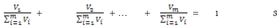
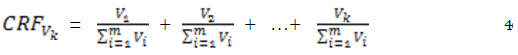
Since the values of V on the horizontal axis are cumulative, Equation 3 indicates that the last value on the horizontal axis must be equal to 1; therefore the maximum value on the horizontal axis is 1. Finally, we define the cumulative relative frequency densities for those values (![]() ) as follows:
) as follows:
For a given value, ![]() such that;
such that; ![]() as shown in Equation 4. As indicated earlier, each value,
as shown in Equation 4. As indicated earlier, each value, ![]() for the cumulative values on the vertical axis is less than or equal to 1. Equation 4 indicates that values on the horizontal axis are cumulatively built up by progressively adding values which are less than 1 until we add the last value, which is also the highest value in the relative frequency table.
for the cumulative values on the vertical axis is less than or equal to 1. Equation 4 indicates that values on the horizontal axis are cumulatively built up by progressively adding values which are less than 1 until we add the last value, which is also the highest value in the relative frequency table.
for the cumulative values on the vertical axis is less than or equal to 1. Equation 4 indicates that values on the horizontal axis are cumulatively built up by progressively adding values which are less than 1 until we add the last value, which is also the highest value in the relative frequency table.
Equation 5 shows that the cumulative relative frequency values add up to 1, regardless of how the values are distributed across different classes of economic variable. The implication is that the terminal point of the Lorenz curve must coincide with the line of equal distribution.

Similarly, Let n be the number of observations in each class of economic commodity. The relative frequency density for a particular![]() , say
, say ![]() , is given by:
, is given by:
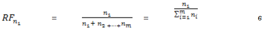
As noted earlier, on the vertical axis we plot the relative frequencies for the number of elements falling within a given class. As seen in Equation 6, we divide a given number of elements in a particular class with the total number of elements for all classes. This will normalize each number to take a value which is less than 1.
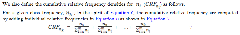
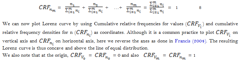
Just like in Equation 5, the cumulative relative frequencies for the number of elements in each class add up to 1 as indicated in Equation 8. As seen in Equation 8 and Equation 5, the highest points on both vertical and horizontal axis coincide at 1 and the lowest points coincide at point 0 (the origin). Equation 5 and Equation 8 indicate that the Lorenz curve coincide with the line of equal distribution from the origin and at the point (1, 1) in the plane. However, between the coordinates (0, 0) and (1, 1), the Lorenz curve deviates away from the Line of equal distribution. The extent of its curvature gives an idea about the extent of inequality in distribution of values of the economic variables under consideration
2.1. Numerical Illustrations – Customer Profitability Analysis
Consider the data in Table 1 below extracted from Hilton and Platt (2014) for the distribution of customers’ income for Patio Grill Company.
For simplicity, we are going to ignore the three customers (107, 134 and 119) who had caused losses to the company. The frequency distribution table below (Table 2) shows the distribution of the remaining profitable customers.
3-Digit Customer Code |
Customer Operating income $ |
Cumulative Operating Income |
112 |
378,530 |
378,530 |
108 |
370,000 |
748,530 |
114 |
351,000 |
1,099,530 |
116 |
340,000 |
1,439,530 |
110 |
336,070 |
1,775,600 |
121 |
331,000 |
2,106,600 |
124 |
330,000 |
2,436,600 |
127 |
300,000 |
2,736,600 |
128 |
281,400 |
3,018,000 |
125 |
276,000 |
3,294,000 |
135 |
270,000 |
3,564,000 |
133 |
251,000 |
3,815,400 |
113 |
219,920 |
4,035,320 |
111 |
205,000 |
4,240,320 |
106 |
199,300 |
4,439,620 |
136 |
82,000 |
4,521,620 |
137 |
35,600 |
4,557,220 |
107 |
(19,050) |
4,538,170 |
134 |
(102,600) |
4,435,570 |
119 |
(119,200) |
4,316,370 |
| Source: Hilton and Platt (2014). |
Class of customers based on profits Profits ($) |
No. of Customers (f) |
0 – 100,000 |
2 |
100,000 – 200,000 |
1 |
200,000 – 300,000 |
6 |
300,000 – 400,000 |
8 |
The total class value can be determined directly from the distribution of customers’ income for Patio Grill Company above. Example for 0 – 100,000, V = 35,600 + 82,000 = 117,600
Profits ($) |
n |
C.F |
v |
C.V |
||
0 – 100,000 |
2 |
2 |
0.117 |
117,600 |
117,600 |
0.026 |
100,000 – 200,000 |
1 |
3 |
0.176 |
199,300 |
316,900 |
0.069 |
200,000 – 300,000 |
6 |
9 |
0.53 |
1,503,320 |
1,820,220 |
0.40 |
300,000 – 400,000 |
8 |
17 |
1.00 |
2,736,600 |
4,556,820 |
1.00 |
Table 3 shows the level of profitability generated by different classes of customers. The number of customers for each class interval of profits are indicated by n and we use it to obtain the cumulative relative frequencies![]() which are plotted on vertical axis. The values, v of profits for each class of customers are the mid points of the class intervals for profits. We then get the cumulative values indicated by C.V and finally Cummulative Relative Values
which are plotted on vertical axis. The values, v of profits for each class of customers are the mid points of the class intervals for profits. We then get the cumulative values indicated by C.V and finally Cummulative Relative Values ![]() which are plotted on the horizontal axis of the curve.
which are plotted on the horizontal axis of the curve.
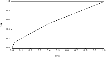
Figure-1. The Lorenz curve for the distribution of customers’ profitability.
2.2. Numerical Illustration – ABC Analysis
Consider the following data extracted from the store records of a certain company
Number of Items |
Total Value |
|||
| Class | No |
Percentage |
UGX |
Percentage |
| A | 1,500 |
10 |
3,750,000 |
75 |
| B | 3,000 |
20 |
800,000 |
16 |
| C | 10,500 |
70 |
450,000 |
9 |
| Source: Lucey (2002). |
Table 4 shows hypothetical data for different classes of inventory adopted from Lucey (2002) with slight modification on the monetary units. The number of items in each class is given in both numbers and percentages. The monetary values of all items in each class expressed in UGX are also given both in numbers and percentages. We used the values in Table 4 to generate key values in Table 5.
2.3. Solution
We have to arrange the monetary value in ascending order as shown in the table below:
| Class | F |
CF |
V |
C.V |
||
| C | 10,500 |
10,500 |
0.70 |
450,000 |
450,000 |
0.09 |
| B | 3,000 |
13,500 |
0.90 |
800,000 |
1250,000 |
0.25 |
| A | 1,500 |
15,000 |
1.00 |
3,750,000 |
5,000,000 |
1.00 |
Table 5 shows the key values generated notably![]() and
and ![]() that have been generated based on the principles laid down in equation 5 and Equation 8 respectively and based on the hypothetical data given in Table 4. We used information in Table 5 5 to draw the Lorenz curve given in Figure 2 below:
that have been generated based on the principles laid down in equation 5 and Equation 8 respectively and based on the hypothetical data given in Table 4. We used information in Table 5 5 to draw the Lorenz curve given in Figure 2 below:
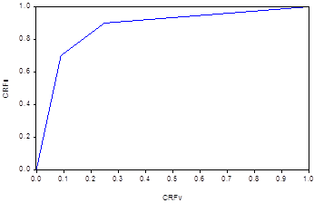
Figure-2. Lorenz curve for the distribution of values of inventory using data from Table 5
The Lorenz curve in Figure 2 above is very far from the line of equal distribution and suggests the very few items in inventory constitute a very high proportion of total value. For example, about 70% of all inventories contribute only about 20% of total value, implying that 80% of total value comes from only about 30% of items in the inventory
3. Conclusion
In this paper, the author proposed further applications of Lorenz curves beyond its original application on examining income inequalities among different classes of individuals. Specifically, the author demonstrated how Lorenz curve can be applied to display heterogeneities in values of some economic commodities. The economic commodities studied here include different classes of items of inventory, something which is a very important issue of management accounting, frequently encountered in accounting for materials. This problem is based on the pareto principle also known as ABC technique of inventory control. The corresponding Lorenz curve for inventory values of different classes of items would guide management on which class of inventory to be accorded more control mechanisms. The second economic commodity examined here are customers, who from management accounting and finance perspectives, are viewed as intangible assets of the firm. All finances that accrue to the firm originate from customers. However, just like any other assets, customers have different values and therefore, some classes of customers are more important to the firm than others, this is based on a well-known principle of 80/20 percent rule in marketing and it is similar to the pareto principles. This situation can be well illustrated using Lorenz curve and management can easily identify the class of customers who are very important for the firm and design appropriate measures of retaining these customers. The paper provided illustrative numerical examples to guide readers.
References
Arcagni, A., & Porro, F. (2014). The graphical representation of inequality. Colombian Journal of Statistics, 37(2Spe), 419-436. Available at: https://doi.org/10.15446/rce.v37n2spe.47947 .
Baek, K. J., Singh, V., & Winer, R. S. (2017). The Pareto rule for frequently purchased packaged goods: An empirical generalization. Marketing Letters, 28(4), 491-507. Available at: https://doi.org/10.1007/s11002-017-9442-5 .
Chakravarty, S. R., Chattopadhyay, N., & D’Ambrosio, C. (2019). Pro-poorness orderings. Review of Income and Wealth, 65(4), 785-803. Available at: https://doi.org/10.1111/roiw.12381 .
Cromley, G. (2019). Measuring differential access to facilities between population groups using spatial Lorenz curves and related indices. T Gis, 23(6), 1332–1351. Available at: https://doi.org/10.1111/tgis.12577 .
Delbosc, A., & Currie, G. (2011). Using Lorenz curves to assess public transport equity. Journal of Transport Geography, 19(6), 1252–1259. Available at: 10.1016/j.jtrangeo.2011.02.008.
Ferreira, F. H., Firpo, S., & Galvao, A. F. (2019). Actual and counterfactual growth incidence and Delta Lorenz curves: Estimation and inference. Journal of Applied Econometrics, 34(3), 385-402. Available at: https://doi.org/10.1002/jae.2663 .
Francis, A. (2004). Business Mathematics and Statistics (6th ed.). Hampshire, U.K: Cengage Learning.
Groot, L. (2010). Carbon Lorenz curves. Resource and Energy Economics, 32(1), 45-64. Available at: https://doi.org/10.1016/j.reseneeco.2009.07.001 .
Gupta, S., & Lehmann, D. R. (2003). Customers as assets. Journal of Interactive Marketing, 17(1), 9-24. Available at: https://doi.org/10.1002/dir.10045 .
Hilton, R. W., & Platt, D. E. (2014). Managerial accounting: Creating value in a dynamic business environment (10th ed.). Penn Plaza, New York: McGraw-Hill Education.
Ibragimov, M., Ibragimov, R., Kattuman, P., & Ma, J. (2018). Income inequality and price elasticity of market demand: The case of crossing Lorenz curves. Economic Theory, 65(3), 729-750. Available at: https://doi.org/10.1007/s00199-017-1037-0 .
Krämer, W., & Neumärker, S. (2019). Skill Scores and modified Lorenz domination in default forecasts. Economics Letters, 181, 61-64. Available at: https://doi.org/10.1016/j.econlet.2019.05.006 .
Lucey, T. (2002). Quantitative techniques (6th ed.). London: Cengage Learning.
Sordo, M. A., Navarro, J., & Sarabia, J. M. (2014). Distorted Lorenz curves: Models and comparisons. Social Choice and Welfare, 42(4), 761-780. Available at: https://doi.org/10.1007/s00355-013-0754-y .
Wang, Z., Ng, Y.-K., & Smyth, R. (2011). A general method for creating Lorenz curves. Review of Income and Wealth, 57(3), 561-582. Available at: https://doi.org/10.1111/j.1475-4991.2010.00425.x.