Testing for the Number of Regimes in Financial Time Series GARCH Volatility 

 

Abdellah Tahiri^1*
Brahim Benaid²
Hassane Bouzahir³
Naushad Ali Mamode Khan⁴

1,2,3ISTI Lab, ENSA, Ibn Zohr University-Agadir, Morocco. 4Department of Economics and Statistics, University of Mauritius, Mauritius.	Abstract This paper investigates the optimal number of regimes that can better describe the corresponding conditional variance to different stock market indices. We compared several GARCH specifications using the Deviance Information Criterion (DIC), provided by the Bayesian approach Markov chain Monte Carlo (MCMC), considering many stylized facts such as asymmetry (i.e., leverage effect), fat-tailed distributions, and volatility clustering. The results show clearly that the four selected models exhibit a leverage effect and have at least two regimes, whatever the GARCH specifications are. In addition, the optimal number of regimes in the conditional variance process may change from a series to another depending on their structure. A predictive test using the Value-at-Risk confirms that the selected processes provide accurate volatility forecasts.
Licensed: This work is licensed under a Creative Commons Attribution 4.0 License.
Keywords: MS GARCH Volatility DIC Model selection Bayesian approach.
Received: 28 January 2021 Revised:  3 March 2021 Accepted: 30 March 2021 Published: 21 April 2021
(* Corresponding Author)

Funding:This study received no specific financial support.

Competing Interests:The authors declare that they have no competing interests.

1. Introduction

Volatility has been a critical element in the risk management world and decision-making. Many mathematicians consider Louis Bachelier as the origin of modern finance (i.e., mathematical finance), particularly the “theory of speculation” thesis (1900). Since that time, several studies have been oriented toward forecasting and modeling volatility. The most popular used class of Auto-regression Conditional Heteroskedastic (ARCH) was introduced by Engle (1982)  and generalized by Bollerslev (1986), gives more flexibility for the conditional variance process structure and allows more capturing to high persistence and clustering of conditional volatility. From a business perspective, negative shocks affect the conditional variance process more than positive ones (i.e., the asymmetry).

Consequently, Glosten, Jagannathan, and Runkle (1993) suggested a new specification (GJR-GARCH) in order to capture the leverage effect (asymmetry) exhibited in the conditional variance process. Different studies have investigated the forecasting difficulties of GARCH model class, such as Hamilton and Susmel (1994) and Lamoureux. and Lastrapes (1993), which mentioned that the GARCH models class might lead to a worse multi-period volatility forecasting than even the constant variance models do. Friedman, Laibson, and Minsky (1989)  highlighted that the weakness of the GARCH class models in forecasting volatility comes from not allowing the conditional variance process to be flexible with “small” or “large” shocks and structural breaks, which can lead to high estimated persistence.

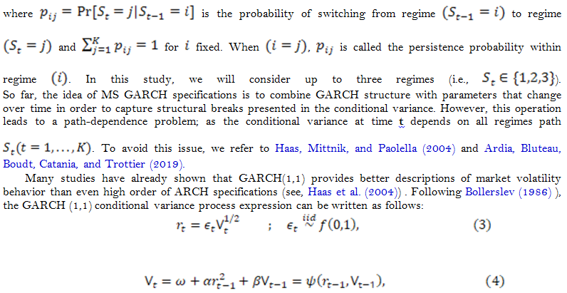
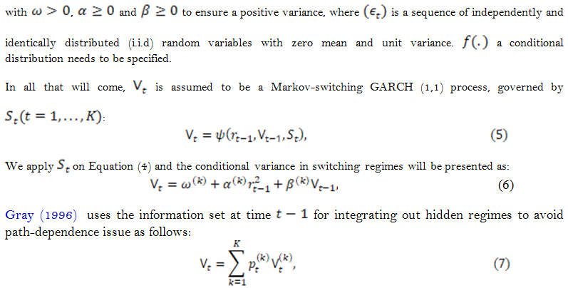
Many researchers have focused on some features of stock market indices. The appropriate model should be able to capture stylized facts observed in financial markets; nonlinearity and asymmetry, for instance. Hamilton (1989) introduced a Markov-switching model to capture structural breaks by allowing conditional variance parameters to switch across different regimes. A way to introduce the “switch” to the return process is provided by the Markov-switching regimes GARCH (MS GARCH) models. These structures can adapt quickly to many variations in the volatility level (Ardia, 2008; Marcucci, 2005).

Using MS GARCH models lead to path-dependence issue. Gray (1996); Dueker (1997)  and Klaassen (2002)  handled this problem through approximation by collapsing the past regime conditional variance. Bauwens, Dufays, and Rombouts (2014)  recommended using the MCMC method to estimate complex models such as MS GARCH, avoiding the path-dependence issue.

In the present paper, we analyze four stock market indices from different financial markets. The primary purpose is to test the optimal number of regimes in volatility presented in each series. The idea was, for different series, the most appropriate model should take into consideration various specifications such as the number of regimes presented in the conditional variance process.

The remainder of this paper is organized as follows: presenting the Markov-switching GARCH (MS GARCH) model in Section 2, while in Section 3, we analyze and investigate about data and the methodology of this work. The empirical results are discussed in Section 4. Finally, Section 5 summarizes the results of this study.

2. Markov-Switching GARCH Model

One of Hamilton and Susmel (1994) ) main recommendations is that ARCH models refer to much persistence in stock return volatility that leads to a poor forecast due to the leverage effect, i.e., the large shocks affect more the volatility than small breaks. The idea to avoid this phenomenon is to allow the ARCH model parameters to change and come from different regimes governed by Hidden Markov Chains (HMC).

By introducing Markov chains on ARCH specifications, we benefit from the primary Markov propriety:

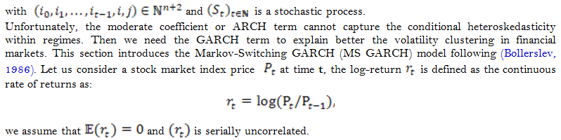
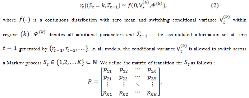
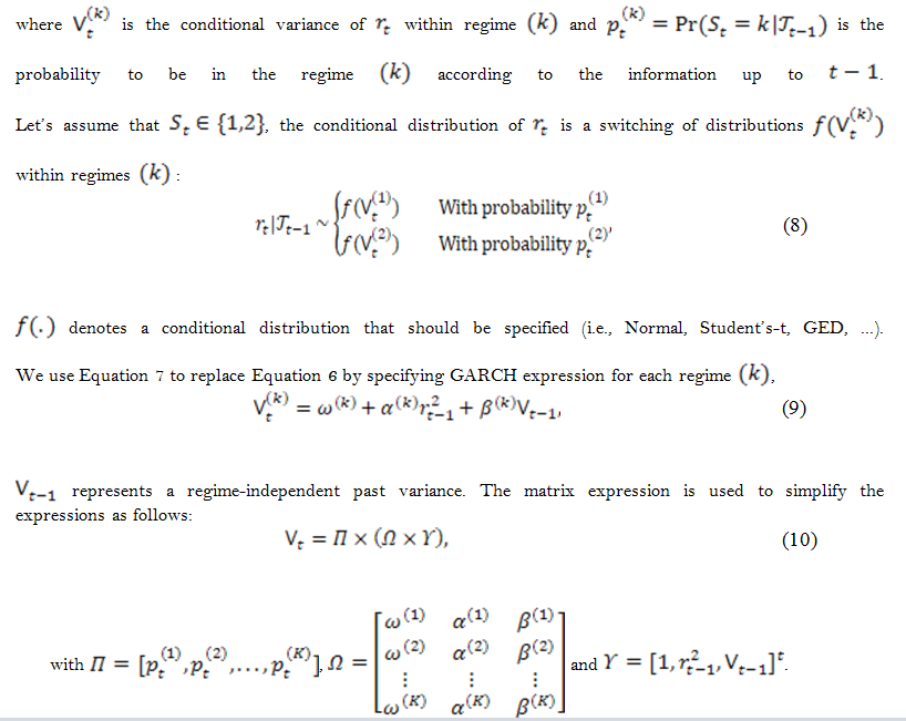
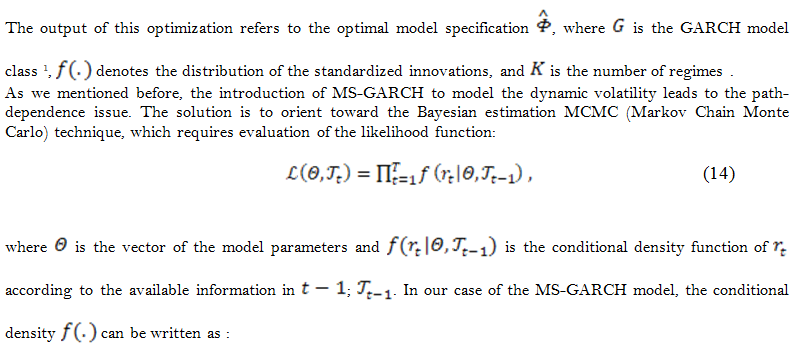
The MS GARCH model following (Ardia, Bluteau, & R̈uede, 2018) can be defined as :

So far, one of the most interesting phenomena in financial markets is what we call the “leverage effect,” caused by the fact that negative returns have an important impact on conditional volatility. However, the standard GARCH (1,1) structure gives the same considerations to negative as positive returns in terms of influencing the future volatility.

To avoid this issue, we will refer to the GJR-GARCH model proposed by Glosten et al. (1993) to capture the asymmetry effect in our time series. The conditional variance process can be expressed as:

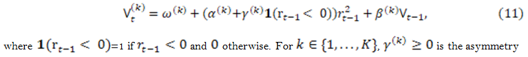
measure parameter in the conditional variance process.
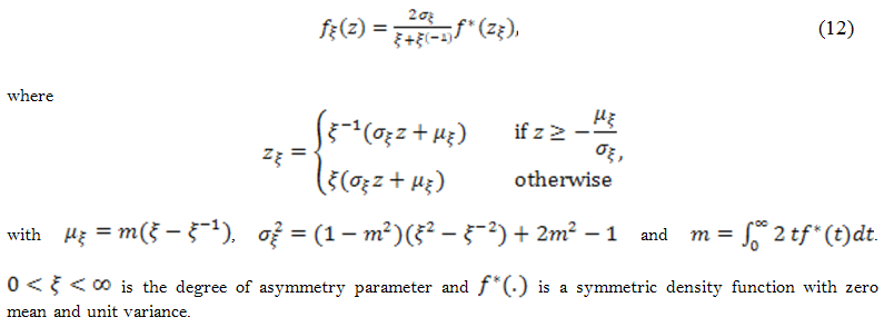
One other dimension which influences the performance of our conditional volatility modeling is the distribution of standardized innovations  that needs to be assumed and specified. In this study, we focus on three distributions, namely, normal, Student’s-t, and generalized error distribution (GED). Regarding the presence of asymmetry, skewed distributions are required. We refer to Fernández and Steel (1998) to define the skewed density as follows:

3. Data and Methodology

In this section, we present the data set used within this study to look at some features that describe the stock market indices series. We selected four major stock market indices, namely, S&P500, FTSE 100, CAC40, and Nikkei 225, respectively, reflecting the USA, UK, France, and Japan markets. All historical data have been obtained from the Yahoo Finance platform. We consider daily log-returns during the period range from January 02, 1990, until October 10, 2019, with around 7,500 observations to ensure that we have captured the maximum of the market behavior. The calculations used the formula;  in percentage, where  is the adjusted-close price at time .

In Figure 1, we plot our series to check the volatility clustering. Clearly, we see that there are “low (high)” fluctuations followed by “low (high)” fluctuations. In addition, the level of changes varies from one series to the other, while the level of changes is more significant for CAC40 and Nikkei 225 series compared to S&P500 and FTSE 100 series. The correlation between the level of fluctuations in log-returns and their stock market index evolution is presented as well.

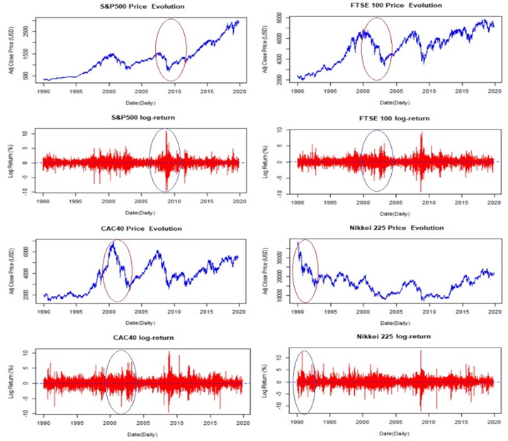
Figure-1. Presentation of stock market indices log-return (%) and price evolution.

Table 1 reports daily log-returns summary statistics for S&P500, FTSE 100, CAC40, and Nikkei 225:

Statistic	S&P500	FTSE 100	CAC40	Nikkei 225
Mean (%)	0.028	0.014	0.013	-0.008
Median (%)	0.053	0.0316	0.035	0.0155
Maximum (%)	10.957	9.384	10.594	13.234
Minimum (%)	-9.469	-9.264	-9.471	-12.111
Std.Dev (%)	1.102	1.082	1.354	1.45
Skewness	-0.264	-0.131	-0.073	-0.149
Kurtosis	8.789	6.17	4.744	5.474
JB-Statistic	24250	12033	7095.5	9169
JB p-value	< 0.01	< 0.01	< 0.01	< 0.01
LM (12)	1972.7	1686.9	1222.6	1282.9
LM p-value	< 0.01	< 0.01	< 0.01	< 0.01

The mean is quite small and close to zero for S&P500, FTSE 100, CAC40, and Nikkei 225 with values of 0.028 %, 0.014%, 0.013 %, and -0.008%, respectively which defend the assumption of keeping the mean zero. The standard deviation (Std.Dev) is around unity. However, the Std.Dev for CAC40 and Nikkei 225 are more important with values of 1.35 % and 1.45% respectively. A high standard deviation indicates high level of volatility (hypothesis to be verified).

The skewness (asymmetry coefficient) is significant and negative showing that the distribution tail spread to the left. The normalized kurtosis (excess kurtosis) is significantly higher than the normal distribution value of 0, indicating that the distributions have fatter tails.

Lagrange multiplier (LM) test demonstrates the presence of ARCH effect in all series, under the null hypothesis of “no ARCH effect”, where  is the number of lags. The results show also that the distributions are far to be normal distributions according to the Jarque-Bera test under the null hypothesis of “normal distribution.”

The main purpose of this paper is to identify the appropriate number of regimes in each series, which better describe the behavior of each stock market index. The idea is to test various models with several specifications, where the number of regimes is one of the parameters that constitute model specifications. Therefore, the optimal number of regimes is that which corresponds to the best specification. We present the optimization problem as follows:

DIC is the Deviance Information Criterion (see Spiegelhalter, Best, Carlin, and Van der Linde (2002)); the model selection criterion.

The estimation of  used the Bayesian approach MCMC based on the adaptive random-Walk-Metropolis sampler (Vihola, 2012) to generate draws from the posterior distribution, where the model parameters are treated as random variables.

The power of MCMC comes from the fact that all inferences are based on the joint posterior distribution of the model parameters. Therefore, normality is not an essential requirement, and the convergence of the estimation algorithm to be judged by ourselves. The posterior estimation accuracy can be evaluated by the Monte Carlo Standard Error (MCSE) for each parameter. The more number of iterations increases, the more posterior estimation accuracy increases (i.e., MCSE →0).

In this study, we generated 20,000 draws, then we discarded the first 5,000 iterations as the burn-in sample, and we considered a lag of 5 to reduce the autocorrelation in the Markov chain. By the end, we built a sample of size 3,000. To ensure the convergence of our model-fitting algorithm, we check the output results with different seeds. ² .

In the present paper, we share the same logic with Box and Jenkins (1976); “all models are wrong. However, some of them are useful”. To compare the fitting-quality of our models, we are using DIC for the Bayesian model selection problems where the posterior distributions of the model parameters obtained by MCMC that can be viewed as the AIC (Akaike Information Criterion) or the BIC (Bayesian Information Criterion):

where,  is the posterior mean deviance that measures the adequacy of fit, while  is the effective number of parameters describing the model complexity (for further details, see Spiegelhalter et al. (2002)).

The DIC is not a criterion to identify the correct model, but it can be used to compare different specifications to determine the most appropriate one since the helpful model is the one with a smaller DIC, which means the goodness of fit is penalized by the model complexity.

4.Empirical Results and Discussion

So far, we have presented the most efficient auto-regression models (i.e., Standard GARCH and GJR-GARCH) with different specifications to get more flexibility in capturing the persistence of the stock market indices conditional volatility. We have also shown the best approach to fit complex models such as MS-GARCH models using MCMC/ Bayesian approach. The suitability of our models is judged with the DIC criterion to select the most appropriate models.

			S&P500			FTSE 100
		k=1	k=2	k=3	k=1	k=2	k=3
S-GARCH	Sk-N	19579.78	19418.08	19450.18	20060.04	19985.1	19981.48
	Sk-STD	19278.53	19272.02	19434.17	19936.01	19936.25	19967.61
	Sk-GED	19250.42	19234.04	19352.87	19947.17	19958.45	19994.52
GJR-GARCH	Sk-N	19320.12	19059.54	19174.34	19882.81	19833.83	19813.35
	Sk-STD	19067.71	19070.24	19028.94	19790.42	19738.61	19945.14
	Sk-GED	19054.8	19014.57	19112.39	19799.58	19798.73	20604.14
			CAC40			Nikkei 225
		k=1	k=2	k=3	k=1	k=2	k=3
S-GARCH	Sk-N	23927.91	23814.4	23777.05	24998.95	24804.86	24789.35
	Sk-STD	23738.48	23738.33	23759.03	24748.38	24733.34	24710.19
	Sk-GED	23764.9	23736.23	23742.65	24760.17	24727.94	24716.21
GJR-GARCH	Sk-N	23734.96	23572.45	23540.55	24827.91	24644.45	24627.53
	Sk-STD	23547.75	23527.04	23512.13	24614.89	24597.53	24585.36
	Sk-GED	23593.04	23552.82	23685.67	24626.19	24599.99	24543.25

In this section, we provide log-returns results analysis of S&P500, FTSE 100, CAC40, and Nikkei 225. In our in-sample analysis, we fit all models (i.e., 4×18=72 models) using the whole data set from January 01, 1990, until October 10, 2019. Before we start fitting models, we filtered our series with AR(1) model recommended by AIC (results not reported) to ensure the uncorrelated between log-returns  observations.

For the four stock market indices, the DIC of different specifications is reported in Table 2. Berg, Meyer, and Yu (2004) and Ardia (2008) have shown many DIC advantages in selecting the adequate model to describe stochastic volatility better.   

For the S&P500 index, almost all two-regimes models provide a better trade-off in terms of fitting adequacy and model complexity, except the GJR-GARCH skewed student’s-t distribution, which can be preferred with three regimes. The comparison leads to select the GJR-GARCH skewed GED distribution model within two regimes that outperform all other specifications.

Regarding the FTSE 100 Index, the skewed student’s-t and GED distributions with single-regime provide more adequacy for the standard symmetric GARCH (i.e., S-GARCH). However, two-regimes GJR-GARCH skewed student’s-t distribution offer once again better adequacy compared to the complexity of the model.

For the CAC40 index, Markov switching GARCH specifications outperform signal-regime. The most appropriate model to describe CAC40 log-returns behaviour is the three-regimes GJR-GARCH skewed student’s-t distribution. In addition, using standard symmetric GARCH requires two-regime specifications.

Finally, for the Japanese stock market index Nikkei 225, as a result of the high market volatility, the comparison has shown that three-regimes are required, whatever the GARCH specifications and the conditional distribution are. In fact, there is an additional advantage for the GJR-GARCH skewed GED distribution model within three regimes.

Table 3, summarizes the results of our comparison. The results show clearly that the MS GJR-GARCH is strongly preferred to describe market stock indices volatility, a justification for the presence of leverage effect.

					Unconditional Probabilities
		Distribution		Regimes	Regime 1	Regime 2	Regime 3	UnVol (%)
S&P500	GJR-GARCH		Sk-GED	K=2	0.7575	0.2425	-	1.031
FTSE 100	GJR-GARCH		Sk-STD	K=2	0.5515	0.4485	-	1.120
CAC40	GJR-GARCH		Sk-STD	K=3	0.3113	0.6766	0.0121	1.955
Nikkei 225	GJR-GARCH		Sk-GED	K=3	0.3494	0.6457	0.0048	1.445

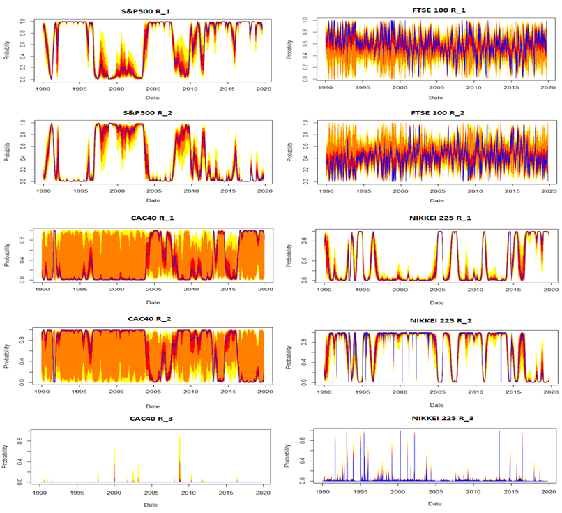
Figure-2. Smoothed probability.

From Figure 2, we can observe that there’s a certain stability in the time within regimes for different series.

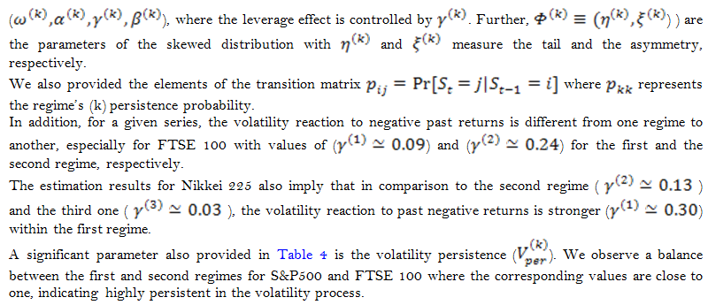
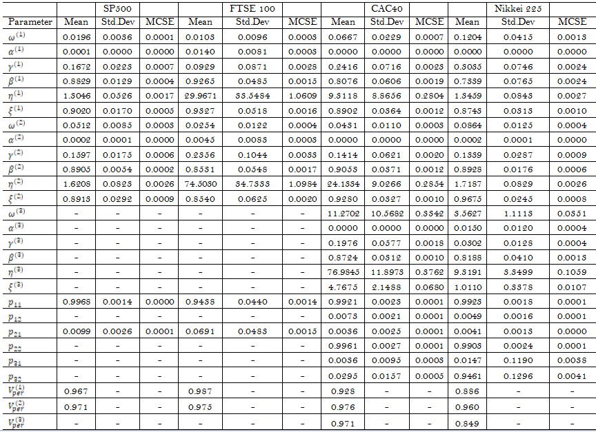
Table 4 presents the parameter estimates of the most appropriate MS GJR-GARCH specifications associated with S&P500, FTSE 100, CAC40, and Nikkei 225; two-regimes skewed GED, two-regimes skewed student’s-t, three-regimes skewed student’s-t, and three-regimes skewed GED, respectively. We report in Table 4, for each stock market indices and a given regime (k), the parameters of GJR-GARCH(1,1);

concerning the Japanese index Nikkei 225. We have developed our regime-switching models that shown high flexibility regarding the persistence of volatility for different stock market indices. Moreover, we would evaluate the performance of the selected models from the out-of-sample analysis point of view. The out-of-sample period started from January 3, 2014, to October 10, 2019, with approximately 1,470 log-returns for each stock market index. A valid model should be able to correctly forecast the Value-at-Risk (VaR) for a specified coverage level. Since we use a family of models that capture time-varying parameters, we consider a wide rolling window to better forecast the one-ahead Value-at-Risk of 5% based on the models selected previously. To test the accuracy of VaR coverage, we refer to the Unconditional Coverage (UC) test of Kupiec (1995)  based on the number of VaR violations (or hit) ⁴, the Conditional Coverage (CC) test of Christoffersen (1998),  and the Dynamic Quantile (DQ) test of Engle and Manganelli (2004) ) founded on the number of violations in addition to the fact that the violation variable  should be distributed independently. Meanwhile, we refer to the Basel Committee on Banking Supervision (BCBS) requirements regarding the internal VaR model validation from a regulatory perspective. The results presented in Table 5 clearly demonstrate the selected model’s ability to predict the VaR accurately at the 5% risk level.

Table-5. VaR Back-Test Results for 95% confidence level.

	Unconditional Coverage		Conditional Coverage		Dynamic Quantile
	uc LRstat	uc LRp	cc LRstat	cc LRp	DQstat	DQp
S&P500	0.0213	0.884	0.3056	0.858	2.3090	0.941
FTSE 100	1.9537	0.162	3.9809	0.137	4.7031	0.696
CAC40	0.1088	0.742	0.8063	0.668	6.3093	0.504
Nikkei 225	0.0736	0.786	1.7790	0.411	10.3516	0.169

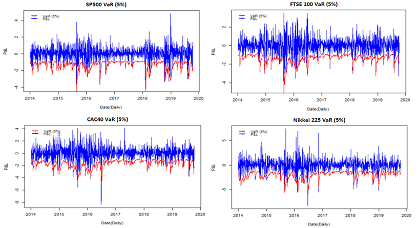
Figure-3. Stock Market Indices Value-at-Risk analysis based on MS GARCH model.

On the other hand, for S&P500 (i.e., the widely popular stock market index), we test the selected model’s forecasting accuracy to predict the VIX index. VIX is the volatility index that represents as closely as possible the implied volatility option based on the S&P500 index. Figure 4, clearly shows the flexibility of the MS GJR-GARCH (1,1) skewed GED distribution model with two regimes in capturing the VIX volatility.

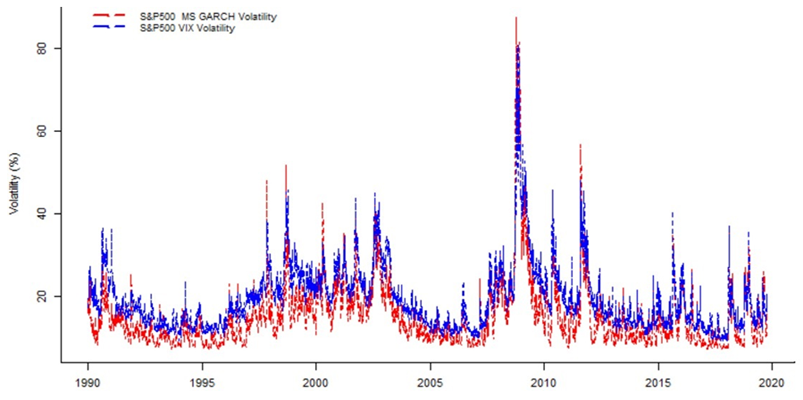
Figure-4. S&P500 MS-GARCH versus VIX volatility evolution.

4. Conclusion

In this paper, we analyzed four stock market indices, namely, S&P500 (USA), FTSE 100 (UK), CAC40 (France), and Nikkei 225 (Japan), based on their daily log-returns from January 1990 until October 2019, about 30 years of data, in order to identify the optimal number of regimes using two GARCH-type specifications; the standard symmetric GARCH (1,1) against the asymmetry GJR-GARCH (1,1), with different skewed conditional distributions (Normal, student’s-t and GED), where all parameters switch across a given number of regimes.

In the empirical part, we estimated models (about 72 models) using the Bayesian approach MCMC avoiding the path-dependence issue. Thus, we provided a simple comparison between these models from the Deviance Information Criterion (DIC) point of view, which measures the model’s adequacy by comparing the fitting quality to model complexity. The stability of estimation is ensured by trying different seeds, where we judge the model’s convergence by ourselves.

Overall, the results revealed that the asymmetry GJR-GARCH outperforms the standard symmetric GARCH (1,1) due to the presence of the leverage effect in the conditional variance process. Moreover, the regime-switching models provide more accuracy than the signal-regime, whatever the specifications are.

Furthermore, the skewed fat-tailed (Student’s-t and GED) distributions are strongly preferred. In addition, the stock market indices, which are characterized by a high level of volatility (CAC40 and Nikkei 225), require three-regimes specifications; low, medium volatility regime, and the third one monitoring the high level of conditional variance with high persistence of volatility.

Finally, the validity of the selected models was verified from the out-of-sample analysis point of view, according to specific statistical tests (i.e., UC, CC, and DQ) in parallel with the Basel committee requirements and the ability to predict the S&P500 implied volatility (VIX).

Based on the empirical results, the main recommendation of the present paper is that the number of regimes in a conditional variance process should be founded on a statistical test and not chosen randomly.

An interesting topic for future research is to apply the results using the marginal likelihood since the DIC is sensitive to the prior distributions.

References

Ardia, D. (2008). Financial risk management with bayesian estimation of GARCH models: Theory and Applications (1st ed., Vol. 612, pp. XIV, 206). Springer-Verlag Berlin Heidelberg: Springer.

Ardia, D., Bluteau, K., & R̈uede, M. (2018). Regime changes in Bitcoin GARCH volatility dynamics. Finance Research Letters, 29, 266-271.

Ardia, D., Bluteau, K., Boudt, K., Catania, L., & Trottier, D. A. (2019). Markov–switching GARCH models in R: The MSGARCH package. Journal of Statistical Software, 91(1), 1-38.

Bauwens, L., Dufays, A., & Rombouts, J. V. (2014). Marginal likelihood for Markov-switching and change-point GARCH models. Journal of Econometrics, 178(3), 508-522. Available at: https://doi.org/10.1016/j.jeconom.2013.08.017.

Berg, A., Meyer, R., & Yu, J. (2004). Deviance information criterion for comparing stochastic volatility models. Journal of Business & Economic Statistics, 22(1), 107-120. Available at: https://doi.org/10.1198/073500103288619430.

Bollerslev, T. (1986). Generalized autoregressive conditional heteroskedasticity. Journal of Econometrics, 31(3), 307-327. Available at: https://doi.org/10.1016/0304-4076(86)90063-1.

Box, G. E. P., & Jenkins, J. M. (1976). Time series analysis: Forecasting and control. San Francisco, CA: Holden-Day.

Christoffersen, P. (1998). Evaluating interval forecasts. International Economic Review, 39(4), 841-862.

Dueker, M. J. (1997). Markov switching in GARCH processes and mean-reverting stock-market volatility. Journal of Business & Economic Statistics, 15(1), 26-34.

Engle, R. F. (1982). Autoregressive conditional heteroskedasticity with estimates of the variance of U.K. inflation. Econometrica 50(4), 987-1008.

Engle, R. F., & Manganelli, S. (2004). CAViaR: Conditional autoregressive value at risk by regression quantiles. Journal of Business & Economic Statistics, 22(4), 367-381. Available at: https://doi.org/10.1198/073500104000000370.

Fernández, C., & Steel, M. F. (1998). On Bayesian modeling of fat tails and skewness. Journal of the American Statistical Association, 93(441), 359-371.

Friedman, B. M., Laibson, D. I., & Minsky, H. P. (1989). Economic implications of extraordinary movements in stock prices. Brookings Papers on Economic Activity, 1989(2), 137-189.

Glosten, L. R., Jagannathan, R., & Runkle, D. E. (1993). On the relation between the expected value and the volatility of the nominal excess return on stocks. The Journal of Finance, 48(5), 1779-1801.

Gray, S. F. (1996). Modeling the conditional distribution of interest rates as a regime-switching process. Journal of Financial Economics, 42(1), 27-62.

Haas, M., Mittnik, S., & Paolella, M. S. (2004). A new approach to Markov-switching GARCH models. Journal of Financial Econometrics, 2(4), 493-530.

Hamilton, J. D. (1989). A new approach to the economic analysis of nonstationary time series and the business cycle. Econometrica: Journal of the Econometric Society, 57(2), 357-384. Available at: https://doi.org/10.2307/1912559.

Hamilton, J. D., & Susmel, R. (1994). Autoregressive conditional heteroskedasticity and changes in regime. Journal of Econometrics, 64(1-2), 307-333. Available at: https://doi.org/10.1016/0304-4076(94)90067-1.

Klaassen, F. (2002). Improving GARCH volatility forecasts with regime-switching GARCH. In Advances in Markov-switching models (pp. 223-254). Heidelberg: Physica.

Kupiec, P. H. (1995). Techniques for verifying the accuracy of risk measurement models. The Journal of Derivatives, 3(2), 73-84.

Lamoureux., C. G., & Lastrapes, W. D. (1993). Forecasting stock-return variance: Toward an understanding of stochastic implied volatilities. The Review of Financial Studies, 6(2), 293-326. Available at: https://doi.org/10.1093/rfs/6.2.293.

Marcucci, J. (2005). Forecasting stock market volatility with regimes witching GARCH models. Studies in Nonlinear Dynamics & Econometrics, 9(4), 1558–3708.

Spiegelhalter, D. J., Best, N. G., Carlin, B. P., & Van der Linde, A. (2002). Bayesian measures of model complexity and fit. Journal of Royal Statistical Society, 64(4), 585–616.

Vihola, M. (2012). Robust adaptive metropolis algorithm with coerced acceptance rate. Statistics and Computing, 22(5), 997-1008.

---

Footnotes: