Determinants of Spot and Forward Interest Rates in Brazil in an International Liquidity Scenario: An Econometric Analysis for the Period 2007-2019 

 

Pedro Raffy Vartanian^1*
Sérgio Gozzi Citro²
Paulo Rogério Scarano³

1,3Adjunct Professor of Economics, Mackenzie Presbyterian University, Brazil. 2Master in Economics, Mackenzie Presbyterian University, Brazil.	Abstract Over the last 25 years, Brazil has been among the countries with the highest interest rates globally. High interest rates have been necessary during several recent times, such as in the period from 1997 to 1999, due to the repeated international financial crises that have plagued the country. From 1999, a sustained path of interest rate reduction begun. With the outbreak of the 2008 international financial crisis, the Brazilian monetary authorities promoted a new round of falling domestic interest rates in response to the recessive effects and the threat of a systemic crisis that could hang over the national financial system. In 2012, a set of interventionist nature policies led to a decrease in the Selic rate. Thus, looking at the last 25 years, it appears that many factors have started to influence the trajectory of Brazilian interest rates. In this context, the present work aims to identify, based on empirical research, the determinants of spot and future interest rates. As a methodology, the research uses a multivariate econometric vector autoregressive model (VAR) with error correction (VEC). The analysis covers the years 2017 to 2019, corresponding to the period in the aftermath of the global financial crisis of 2008. The results evidence that both the spot rate and the DI future can be determined by the fluctuations in the level of inflation and by the level of activity and the real exchange rate, in addition to the effects of the lagged variables themselves.
Licensed: This work is licensed under a Creative Commons Attribution 4.0 License.
Keywords: Monetary policy Interest rates The 2008 crisis VAR Model. JEL Classification C40; E40.
Received: 10 June 2021 Revised:  15 July 2021 Accepted: 19 August 2021 Published: 2 September 2021
(* Corresponding Author)

Funding: This work has been supported by grants from the Mackenzie Research Fund (MackPesquisa).

Competing Interests:  The authors declare that they have no competing interests.

1. Introduction

The main instrument of monetary policy is the basic interest rate; its importance is derived from the scope of the effects it exerts on the economy. Generally speaking, high interest rates reduce aggregate demand, slow down the economy and reduce inflation, while lower interest rates increase aggregate demand, heat up the economy and put pressure on inflation. High interest rates were necessary, especially in the initial years of the Real Plan, from 1994 onwards, as they were combined with a fixed and valued exchange rate regime and served as an anchor for the consolidation of the stabilization plan implemented at that time.

From 1997 to 1999, emerging countries’ financial markets were plagued by successive financial crises, such as the Mexican (1994), Asian (1997), Russian (1998) and Brazilian (1999) crises. Amid recurring external crises, the exchange rate band regime came to an end, causing the Brazilian monetary authority to replace it with the inflation targeting regime, which granted greater freedom to monetary policy and provided a sustained trajectory of reduction in the rate of fees. However, the domestic interest rate was kept high, as it started to reflect the sum of the international interest rate and the risk premium. The risk premium, in turn, reflected the worsening of the domestic balance of risks resulting from the “blackout” of energy, the resurgence of inflation and the political uncertainties arising from the end of the presidential cycle represented by the Fernando Henrique Cardoso government.

As of 2003, domestic interest rates began a new phase of reduction. Considering that the differential in relation to international rates remained high, the Banco Central do Brasil (BCB) adopted a strategy of strengthening international reserves. At the same time, Brazil entered a virtuous cycle characterized by austere fiscal policy, the consolidation of the inflation targeting regime, the maintenance of consecutive primary fiscal surpluses and the recovery of the monetary authority’s credibility. Amid the recovery of Brazilian macroeconomic credibility, the outbreak of the international financial crisis in 2008 did not prevent further declines in domestic interest rates as a response to the recessionary effects and the threat of a systemic crisis that hovered over the national financial system. However, in the period 2011/2012, these pillars of economic policy were replaced by the New Economic Matrix (NEM), supported by a set of expansionist and interventionist fiscal policies, which led to a “forced” reduction in the Selic rate at a time of inflationary acceleration. As a result, in 2013 it was necessary to again tighten monetary policies and interrupt the downward trend in interest rates.

Over the last 25 years, it thus appears that many factors were determinants of Brazilian interest rates. These can be grouped among those that explain them through the hypothesis of rational expectations and efficient markets, or through the influence of economic variables, as will be subsequently discussed. In light of the contributions of these works, the main objective of this article is to empirically explain the determinants of interest rates. The justification for this analysis lies in the identification of new patterns of influence on interest rates, especially after the 2008 international financial crisis and its effects on international monetary conditions caused by the Quantitative Easing program in the US.

In this context, this article is organized into five sections, in addition to the introduction. The next section contemplates the theoretical framework, with an emphasis on the relationship between the spot rate and the future interest rate and their respective determinants according to economic variables. In section 3, the historical context is presented, focusing on the inflation targeting regime and the influence of the 2008 crisis, whereas in section 4, the methodology used is presented and the variables to be studied are specified. Finally, section 5 analyzes the results obtained in light of the theory developed, followed by the final considerations in section 6.

2. Theoretical Review

The Selic rate is the basic interest rate of the economy, the main monetary policy instrument possessed by the Central Bank of Brazil (BCB). Selic was created in the early 1980s and its calculation is based on the averages of one-day financial transactions, backed by federal government bonds with a counterparty from the BCB. Similarly, there is the interbank deposit rate (DI), a reference in the issuing of the Interbank Deposit Certificate (CDI). It is formed by the weighted average of 1-day interbank transactions, calculated by the Central for the Custody and Financial Settlement of Securities (Cetip). The basic difference between the Selic and the DI rate is the counterparty of the transactions. In the first, a bank negotiates directly with the BCB; in the second, the banks themselves negotiate with each other. Both Selic and DI transactions fail to reflect the credit risk of counterparties, but the opposite is true of the liquidity conditions of the economy, according to Oliveira and Ramos (2011).

In view of the time horizons, the risks and uncertainties of the spot market on investors and the need to find ways to protect against fluctuations in the economic cycle, the macroeconomic literature tries to explain the relationship between short-term interest rates and their long-term counterparts. According to Tabak and Andrade (2003), central banks control short-term interest rates, but aggregate consumption and investment decisions are generally seen as being related to long-term interest rates. In Brazil, long-term rates are negotiated through DI futures contracts, whose underlying asset is the average daily rate of interbank deposits, as calculated and published by the Futures Exchange. The contract has a principal amount of R$100 thousand on the expiration date and the amount on the trade date, known as the unit price (PU), which is equal to the amount of R$100 thousand discounted at the negotiated rate. The rate used for the discount reflects the expected evolution of the DI, that is, the transformation into PU through the expectation regarding the future interest rate.

Silva and Holland (2013) analyze the dependence of price and interest rate formation in the government bond market in relation to the DI future. In this study, DI future curves are used as references for the pricing of government bonds, which is a peculiarity in the formation of fixed interest rates in Brazil. The authors test the causality and dependence of the interest rate on DI futures using the Granger method with the expectation that the spot market for government bonds will cause (in Granger's sense) the DI futures market, but the empirical evidence indicates that the bid-ask spread of the “Granger DI futures” market causes the bid-ask spread on government bonds, and not the other way around, as one might expect.

Barbosa (2006) addresses the interaction between monetary policy and public debt management to understand the determinants of interest rates by economic variables and starts from a model that analyzes two markets: bonds issued by the Treasury indexed to the Selic rate and bank reserves deposited at the BCB. Bank reserves are backed by government bonds and have a wholly inelastic demand curve, as bonds and reserves are perfect substitutes. On the other hand, the demand curve for Treasury bonds is positively sloping, as an increase in the Selic rate increases demand for these bonds. Assuming a reduction in the Selic rate is below the equilibrium rate, there is an excess supply of Treasury bonds, which translates into an excess supply of bank reserves. As this is a Selic-indexed bond market, it remains for the BCB to acquire this excess supply of reserves, otherwise the interest rate would drop to zero. On the other hand, assuming an increase in the interest rate above the equilibrium rate, the excess demand for Treasury bonds leads to a shortage of bank reserves, leading the BCB to intervene in the market to prevent the interest rate from rising abruptly. Consequently, for Barbosa (2006), the perception by agents of a risk premium arising from the rollover of the Brazilian public debt by the BCB is the reason for the high interbank interest rates, which in turn is reflected in the Selic. The risk premium implies a connection between BCB funds and Treasury bonds that influence the economy's basic interest rate.

Franco (2011) discusses the existing connection between the management of the Brazilian fiscal imbalance and monetary policy as a determining factor for interest rates and points out that the interest rate needs to be kept permanently high to finance the fiscal imbalance, via public debt rollover, due to a distributive conflict between the public sector and the private sector for national savings (crowding out). Furthermore, Franco (2011) also considers the influence of the overnight market design, with a concentration of business in Financial Treasury Bills (LFTs), which, as they are indexed by the Selic rate, create issuance difficulties for other Treasury bonds, as well as long-term private issues, with the exception of short pre-fixed issues. As a result of this, the risk of debt intermediation between the Treasury and the public that finances it increases, with the strengthening of a mutual fund industry, separate from the banks and, at the same time, financed by them, whose objective is to load public debt, as if it was interest-bearing demand deposits.

In their research, Barbosa (2004) assesses that the inertial behavior of the interest rate may have a determining effect on Brazilian interest rates. Interest rate inertia is described as the change in the interest rate proportional to the difference between the desired and actual interest rate. For the analysis, it uses the Taylor Rule (RT) as a theoretical model. The RT is a reaction function in terms of the interest rate, being an important variable in the natural interest rate. As it was estimated for different countries and times, its standard econometric specification must contain at least three variables: the lagged interest rate, the inflation gap and the output gap. Assuming that the central bank reduces the inflation rate target, keeping the inflation rate stable in the initial moment will increase the real interest rate, leading the economy down a recessive path. Assuming again that the central bank reduces the inflation rate target, but concentrating on inertial behavior, the inflation rate will start to gradually fall and the real interest rate will tend to increase until it reaches its maximum point.

Again, Barbosa, Camêlo, and João (2016) analyze the determinants of the real interest rate in Brazil through the adaptation of RT to the Brazilian economy. Under the monetary policy rule, the interest rate must increase if there is an increase in the difference between the nominal natural interest rate and the current interest rate if inflation expectations are above the target, if the real output is above the potential and if currency depreciation occurs.  Barbosa et al. (2016) define the natural interest rate as being given by the sum of the real interest rate, sovereign risk and exchange risk. Thus, the real interest rate would be explained by four factors: 1) international interest rate; 2) foreign exchange risk premium; 3) country risk premium; and 4) Treasury Financial Bills (LFTs) premium.

Prado and da Silva (2017) test how the determination of the interest rate can be influenced by other aspects besides the price level variation, such as economic growth and public indebtedness. The results of the estimations performed by autoregressive vectors (VAR) are evaluated through impulse response functions. Thus, when the origin of the shock is in the inflation deviation, the response in the interest rate contrasts what is expected, that is, there are reductions in the interest rate. When the shock originates in public indebtedness, the effect occurs as expected, however, in a less intense way than the shocks verified in the current inflation deviation and in the output gap. The output gap shock has an effect similar to that observed in the current inflation deviation shocks. Finally, the shock to current inflation has a positive response, but is more significant after the fifth month. When the shock is registered in exchange rate fluctuations, the result is practically nil in the interest rate.

Segura-Ubiergo (2012) also points out the fiscal issue as one of the determinants when studying why Brazil has relatively high real interest rates in comparison with other emerging countries. The estimation is done via Ordinary Least Squares (MQO) or via Generalized Moment Methods (GMM). In short, increases in private and public savings rates (reductions in fiscal and external deficits) are associated with reductions in the real interest rate. Furthermore, it observes the increase in the real interest rate when inflationary volatility occurs. The study also identifies that an increase in the US interest rate (Fed Funds Rate) of 1 percentage point (pp) is associated with an increase in the real interest rate of 0.3 pp in the short term and 0.5 pp in the interest rate.

In this context, considering the theoretical review and the results already found in relation to impacts on spot and future interest rates, the next section will contemplate the methodology, addressing both the variables and the model to be used in order to answer the research question.

3. Historical Evolution and Determinants of the Brazilian Interest Rate

In this section, the historical evolution of the determinants of interest rates in Brazil is developed. The domestic debt financing mechanism, the implementation of the inflation targeting regime and the influence of external factors are addressed, with an emphasis on the 2008 international financial crisis, which has a decisive role in the analysis, given that it gave rise to expansionist monetary policies adopted by central economies in order to combat recessive effects. Such expansionist policies had a fundamental effect on changes in international liquidity patterns. In particular, in the US, the package of measures was marked by Quantitative Easing (QE), which consisted of government bond repurchase operations of around USD 85 billion a month, with the aim of injecting liquidity into the US economy and forcing a reduction in the long-term interest rate.

For Barbosa (2006), interest rates are historically high in Brazil due to a structural problem arising from the domestic financing mechanism of the securities debt. In the early 1970s, when the open market for securities (open market) and the BCB bank reserve market were created, there was no secondary market for the trading of government bonds. The bonds issued by the Treasury were the so-called Adjustable National Treasury Bonds (ORTN); these were not traded on the open market by financial institutions. The BCB, as a way of operating in the open market and improving public debt management, created National Treasury Bills (LTNs), which were issued by the Treasury. In the 1980s, with the introduction of the new settlement and payments system (SELIC) for government bonds, the exchange of bonds for BCB funds began to take place on the same day. As a result, Treasury bonds and BCB reserves became almost perfect substitutes as a store of value. In 1986, the BCB started to issue bonds indexed to interest rates in the overnight market. Since then, this security has served as backing for open market trading, as, in addition to being free from the risk of interest rate fluctuations, it has allowed for the creation of liquidity reserves for the national banking system. This monetary policy arrangement was vital to avoid the dollarization of the Brazilian economy during the period of hyperinflation, because it enabled the banking system to create reserve funds, backed by government bonds, with full liquidity from the BCB reserves. On the other hand, the financing of the securities debt, based on bonds indexed to the interbank interest rate, started to include a risk premium for the rollover of public debt. In this context, the debt financing mechanism as a determinant of interest rates is also critically analyzed by Franco (2011), mainly because it is considered to be a “captive market” for the rollover of public debt. The internal debt, concentrated in LFTs, indexed by the Selic rate and almost without credit risk, is automatically rolled among local creditors and works as an indexed quasi-currency designed to avoid the transfer of the financial wealth of the economy. This gives rise to a mutual dependence between the Treasury and the mutual fund industry, whose objective is to carry public debt as if it were made up of interest-bearing demand deposits. Segura-Ubiergo (2012) highlights the history of volatility and accommodation and their persistently high levels of inflation as one of the reasons for the high Brazilian real interest rates. In the 1970s, annual inflation was moderately high, averaging 30% per year, rising to exceedingly high levels in the 1980s, with an annual average of 200%, turning into hyperinflation between 1989 and 1994, with an average of 1,400 %. In this scenario, a strong correlation was observed between high inflation rates and high real interest rates, often used as the only instrument to combat hyperinflation. When analyzing the drop in real Brazilian interest rates between January 1997 and June 2012, Pessôa (2013) argues that the reduction was due to a cyclical phenomenon, as a consequence of the 2008 financial crisis, which resulted in severe recessions in developed countries. In addition, the Brazilian investment rate, which in the period from 2004 to 2008 grew at a faster pace than the savings rate, started to decelerate from the third quarter of 2010 onwards. Thus, the reduction of the real interest rate also responded to this downward movement in the investment rate of the economy. However, low real interest rates allowed inflation to accelerate, requiring a reversal of monetary policy that resulted in one of the biggest recessions in the Brazilian economy, as shown by Vartanian and Garbe (2019).

In line with the observation of possible causes for the fall in the real interest rate, Gottlieb (2013) highlights the reduction in the interest rate in the main developed economies since 2008 and the structural changes that occurred in the Brazilian economy such as the Fiscal Responsibility Law, the improvement of the fiscal situation, the consecutive primary surpluses, the increase in domestic savings and the full effectiveness of the inflation targeting system. Regarding the importance of the inflation targeting regime, it is worth mentioning that, after its introduction in early 1999, the Selic rate dropped from a level above 40% per year to just 15% in January 2001, as illustrated in Figure 1.

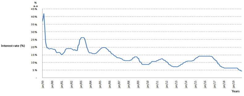
Figure-1. Evolution of the Selic rate as a % per year from 1999 to 2019.

According to Barbosa-Filho (2008), the good functioning of the target regime was one of the determinants of the observed decline. From 1994 to 1998, the annual average of the real basic interest rate was 21.9%. Between 1999 and 2006, this average dropped to 10.7%. Thus, with regard to interest rate reduction, Prado and da Silva (2017) state that the inflation targets did not represent a rigid policy rule alone, but rather a clear and transparent governance structure for the monetary policy that allowed the authorities to act effectively in the control of inflation, with gains in managing expectations and in reducing the basic interest rate.

A new cycle of interest rate reductions was observed from 2008 onwards, during which time the Brazilian economy was hit by the effects of the shocks arising from the international financial crisis that year. According to Kindleberger and Liber (2013), three elements contributed to the crisis. First, the monetary policy employed by the Federal Reserve (Fed) in the period preceding 2007. The large reduction in the US base interest rate was the response employed by the Fed to combat the effects of the previous crisis, which occurred in March 2000, restricted to the local scope and called the “dot.com” crisis. As of January 2001, the interest rate, which was at 6.5%, was gradually reduced until it reached 1.7% in 2002 and 1.5% in 2004. Secondly, the increase in liquidity stimulated the capacity to consumption, resulting in a strong boost in the construction industry and the mortgage market. Subsequently, the deregulation of financial markets under the Democratic and Republican administrations of Bill Clinton and George W. Bush, respectively, contributed to the dismantling of regulatory mechanisms and the emergence of a complex, diversified and poorly regulated financial market that contained the ideal seeds for the germination of the crisis in 2007. Thirdly, as a result of deregulation, the mortgage financial market and, in particular, mortgage instruments, namely subprime, were related to the housing bubble and the belief that house prices would follow an indefinite uptrend.

The first effects of the international financial crisis emerged in 2007, marked by successive financial crashes and announcements of spectacular losses in prestigious investment properties around the world. The crisis in US subprime mortgage market, initiated by a series of defaults on risky loans, spread to credit markets on an international scale. In the Brazilian economy, the contagion was more accentuated from the second half of 2008 onwards. Brazil, in particular, although not at the epicenter of the crisis, felt the contagion in the form of capital flight, restrictions on access to external sources of credit, falls in commodity prices, pressure on the exchange rate and reductions in interest rates. According to Blanco and Holanda (2010), from September 2008 to March 2009, the São Paulo Stock Exchange, the main stock market in the country, registered a fall of 25%, spreads that measure sovereign risk increased by 77% and the real interest rate depreciated by 40%. A wave of defaults resulted in the growth of so-called “non performing loans” (NPLs), increasing cash pressure and generating a run on smaller banks. Domestic credit, which until then had shown monthly growth of 2% to 3% since 2005, slowed down to 0.2% in January and 0.1% in February 2009. Through the external trade channel, the drop in global economic activity reduced commodity prices by more than 30% and demand from the foreign market for Brazilian products by more than 40%. In the real economy, after 12 consecutive quarters of expansion, GDP contracted by 3.4% in the fourth quarter of 2008 and 1% in the first quarter of 2009 due to the reduction in the supply of credit, which interrupted the growth trajectories’ demand for investment and durable goods. At the sectoral level, industrial production plummeted 8% in the last quarter of 2008, with an additional drop of 3.2% in the first quarter of 2009, resulting in an accumulated drop of 12% in the first two quarters after the outbreak of the crisis.

The effects of the global crisis required responses from the Brazilian monetary authority. According to Blanco and Holanda (2010), the good reputation enjoyed by the BCB in controlling inflation facilitated the adoption of an aggressive interest rate reduction strategy. Inflation indicators at moderate levels combined with the economic slowdown made room for a drop of 500 pp in the Selic rate, from 13.75% in September 2008 to 8.75% in July 2009. It is in this context, therefore, that this work aims to test that the significant impact on the world economy, especially in liquidity conditions, has contributed to the trajectories of spot and future interest rates observed in Brazil since then.

4. Methodology

Given the evidence of a strong fall in the Selic rate between 2008 and 2009, as a result of the consequences of the 2008 financial crisis, this paper applied the VAR methodology with error correction (VEC). The main advantage of the VAR model is the possibility of estimating several variables simultaneously, avoiding the problems with identifying parameters in multi-equational models. It is an appropriate model when one is not completely sure about the endogenous nature of one variable in relation to the others. The advantage is to consider all endogenous variables, avoiding the subjectivity of the decision on which will be endogenous or exogenous. It also extends the autoregression from one variable to multiple time-series variables, that is, to a vector of time-series variables. When applied, it can develop a single model that is capable of predicting all variables, resulting in mutually consistent predictions.

One of the assumptions of regression models is that the series are stationary. A series is stationary if it presents a constant mean and variance over time. Stationarity requires that, in a probabilistic sense, the future is equal to the past. Otherwise, the series is non-stationary. One way to treat non-stationary variables is to find linear combinations of stationary integrated variables, called cointegrates. If two series, for example Xt and Yt, are cointegrated, it means that they present an equal or common stochastic trend, eliminated by means of the difference Yt – θXt. If Xt and Yt are cointegrated, their respective first differences can be modeled using a VAR, augmented by the inclusion of an additional regressor Yt-1 - θXt-1. This is called an error correction term. By combining the VAR with the error correction term, the model known as the error correction vector (VEC) emerges. In this model, past values of Yt – θXt help to predict future values of ΔYt and ΔXt. According to Vartanian (2010), the solution of cointegration is a key factor in solving problems related to non-stationary series.

The variables used in this research are subsequently described and were selected in order to understand the relationship between the observed shocks and changes in the Selic and DI future interest rates. The series were of a monthly frequency and were collected in the period between 2007 and 2019:

i) Selic basic rate, identified by interest rate, IR, represents the basic interest rate of the Brazilian economy, Selic Over, set during a meeting of the Monetary Policy Committee (Copom) and used as an index for government bonds. The series of the variable was obtained from the BCB;

ii) the broad national consumer price index (IPCA), identified by INFL, aims to measure the inflation of a set of products and services sold in retail, referring to the consumption of families with incomes between 1 and 40 minimum wages, in addition to its use by the BCB as a reference for the inflation targeting system. The IPCA was sourced from the Brazilian Institute of Geography and Statistics (IBGE);

iii) the seasonally adjusted monthly index of economic activity, represented by the Economic Activity Index (IBC), aims to measure the contemporary evolution of the country's economic activity. The series was obtained from the BCB;

iv) country risk, based on sovereign debt securities issued by Brazil in the international market, identified as EMBI and calculated by JP Morgan, which calculates the financial returns obtained above those issued by the US Treasury (T-Bond), in addition to an indication of the degree of confidence of investors in the country. The source of the data is JP Morgan;

v) future average rate of one-day interbank deposits, represented by F_IR, has as an underlying asset the average daily rate of interbank deposits and presents a proxy of the future interest rate, record high liquidity and absence of credit risk. The series was obtained from the BCB;

vi) the effective federal funds rate, the main US interest rate, identified as FFR, defined by the Fed through its monetary policy committee, equivalent to the Selic rate. It is the rate at which commercial banks and other institutions lend excess reserves to other interbank market participants. The source of the series is the Federal Reserve;

vii) public sector net debt indicator, identified as DEBT, represents the debt/GDP ratio as a % and refers to the accumulated flow over 12 months and incorporates all levels of government (Federal, State and Municipal). The debt/GDP ratio was sourced from IPEADATA;

viii) the real exchange rate, represented by RER, refers to the nominal exchange rate adjusted by the difference between the price levels practiced in the international and domestic market and is calculated by IPEA based on a weighting of the participation of the Brazilian economy in the commercial exchange in relation to the main trading partners. The source of the series is IPEADATA.

Table 1 presents the descriptive statistics of the presented variables and the results of the normality tests. According to the usual procedure found in the literature of VEC models, the econometric analysis starts with the level series and applies the logarithmic transformation only to series that are not presented as rates, since the VEC model calculates the first difference of the series. To perform the calculations, tests and estimates, Gretl and Eviews software were used.

	F-IR	IR	INFL	FFR	DEBT	EMBI	IBC	RER
	(%)	(%)	(%)	(%)	(% PIB)	(b.p.)
Average	10.20	10.18	0.45	1.01	40.53	256.43	136.77	120.59
Median	10.73	10.66	0.44	0.19	38.99	239.00	137.80	119.09
Maximum	14.28	14.15	1.32	5.26	55.70	523.00	148.70	163.34
Minimum	4.45	4.40	-0.23	0.06	30.00	142.00	119.44	91.41
Standard deviation	2.61	2.65	0.28	1.42	7.59	78.74	7.30	17.25
Jarque-Bera	8.40	7.94	11.44	120.93	11.76	57.12	8.77	7.33
Probability	0.01	0.02	0.00	0.00	0.00	0.00	0.01	0.02
Number of observ.	156	156	156	156	156	156	156	156

According to Table 1, the interest rate in place in Brazil has always been high when compared to international standards. Between 2007 and 2019, the average rate reached 10.19% per annum (pa) versus the average for the US base interest rate of 1.02% pa. The volatility of the Brazilian interest rate was equal to 2.66x, almost twice as high as the volatility of the US base interest rate (1.42x). In the same period, the monthly inflation rate peaked at 1.32%, resulting in an average real interest rate of 10.72%.

The volatility of the country risk series, measured by the standard deviation, was also higher than the others (78.75x), and reached a maximum value in December 2015 due to the political crisis caused by the impeachment process of President Dilma Rousseff. Based on Table 1, the Jarque-Bera test pointed to the absence of normality in the tested variables. The non-normality of residuals in analyses of Brazilian macroeconomic series is common in studies that use the Jarque-Bera test, as attested by Minella (2001), Pinheiro and Amin (2005) and Oreiro, Paula, Silva, and Ono (2006). The results are not an obstacle to the interpretation and analysis of the data because the first difference method will be applied to the variables in the VEC model.

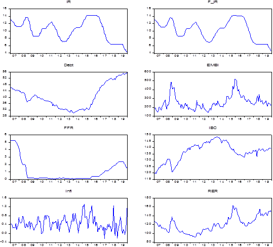
Figure-2 . Level variables from 2007 to 2019.

Figure 2 illustrates the evolution of the variables between 2007 and 2019. We identified that the period prior to 2008 was one of strong expansion of economic activity in Brazil. With the outbreak of the international crisis and the US interest rate being reduced to levels close to zero, and maintained over the next seven years, one of the effects observed was the drop in the Selic rate in the same direction by the future interest rate. At the same time, the real exchange rate began an appreciation trajectory until 2011, which was followed by a long period of devaluation between 2012 and 2015. From 2008 to 2011, the global recessionary scenario caused significant global deflation. The maintenance of the high differential between the Selic and the international interest rate determined a large flow of resources to Brazil and contributed to the appreciation of the nominal exchange rate. In 2012, during the first term of President Dilma Rousseff, the basic interest rate was reduced again, but the domestic scenario pointed to an increase in prices. Still considering the economic stagnation of the main developed economies, the real exchange rate began a movement of depreciation, accelerated by the political uncertainties that dominated the political scenario at the time. These uncertainties peaked in 2015, on the eve of President Dilma Rousseff's impeachment process. With the beginning of Michel Temer's presidential term, from 2017, there was a slight depreciation of the real exchange rate, especially after the episode in which a recording with the then president of the Republic, Michel Temer, was released, with adverse effects in the stock and exchange markets on the date popularly known as “Joesley Day”, which compromised the future reform agenda, especially the pension reform. Although the public debt indicator maintained an upward trend, declining interest rates and country risk stability around 250 basis points (p.b) were once again observed. As of 2018, with the beginning of the presidential campaign, the nominal exchange rate started to register new and successive devaluations, contributing to the new depreciation of the real rate.

To assess the stationarity of the series used, we considered a necessary prior procedure for the precedence tests, the Dickey-Fuller unit root tests, as shown in Table 2. The unit root identification procedures were performed using Gretl software with testing of up to 12 lags, considering the intercept and trend components. The column identified as p-asymptotic reveals the probability of not rejecting the null hypothesis of the presence of a unit root. Clearly, only the FFR (US interest rate) series was stationary. On the other hand, and still according to Table 2, all other series were shown to be stationary in first difference according to the ADF test.

Variables	Lags	Constant	Trend	Tau statistic	p- value	Significance
IR	6	Yes	Yes	-1.94	0.63
F-IR	4	Yes	Yes	-2.27	0.45
DEBT	3	Yes	Yes	-0.89	0.96
EMBI	0	Yes	Yes	-2.61	0.28
FFR	8	Yes	Yes	-5.77	0.00	***
IBC	2	Yes	Yes	-2.07	0.56
INFL	8	Yes	Yes	-2.72	0.23
RER	3	Yes	Yes	-2.94	0.15
D_IR	5	Yes	No	-4.21	0.00	***
D_F-IR	4	Yes	No	-3.77	0.00	***
D_DEBT	0	Yes	No	-10.75	0.00	***
D_EMBI	0	Yes	No	-11.65	0.00	***
D_IBC	1	Yes	No	-7.10	0.00	***
D_INFL	7	Yes	No	-8.50	0.00	***
D_RER	0	Yes	No	-9.57	0.00	***

Note: *** Rejection of the null hypothesis of unit root at the 1% level of significance.

Based on Table 2, it is possible to reject the null hypothesis of the presence of unit roots for the series in first difference with p-asymptotic less than 1%, except for the US interest rate variable, which shows stationarity at such a level. In general, a series presents a stationary behavior when its p-value is less than 5%. As practically all series are non-stationary, the VEC model, in detriment of the VAR model, should be used to estimate the impulse response functions.

Once the issue of non-stationarity of the series is solved with the application of the VEC model, the next test consists of identifying the optimal number of lags. Such a procedure is necessary due to the presence of autoregressive components. The increase or decrease in the number of lags can lead to instability and the loss of predictive power. For the VEC model, two selection criteria were applied: Akaike (AIC) and Schwarz (SC); tests located in the interval between 1 and 5 lags were also performed, as an exaggerated number would imply a loss of degrees of freedom. On the one hand, models with few lags can have bias problems due to the omission of relevant variables. On the other hand, including more variables than necessary can lead to the problem of irrelevant variables. In order to not choose the number of lags arbitrarily, tests were performed based on different lag estimates that changed the identification of the number of cointegration equations. The results are reported in Table 3. Tests for choosing lags are discussed in detail in Lütkepohl (1991).

Models	Cointegration equation	Lags	Akaike	Schwarz
1	3	1 a 1	-21.0576	-18.6911*
2	3	1 a 2	-20.9964	-17.3520v
3	2	1 a 3	-21.1976	-16.5822v
4	3	1 a 4	-21.0265	-14.7921v

The AIC and SC criteria were used with the aim of finding the most parsimonious model, with the minimum parameters that accurately explain the behavior of the response variable. Both criteria use the maximum likelihood function as a measure of adjustment, and smaller values ​​are preferred, as the value of the criterion rises as the sum of squares of the errors increases. Table 3 includes the column with the number of cointegration equations, according to the Johansen (1991). During the procedure, the number of cointegration equations was changed as the number of lags was similarly altered. According to the AIC criterion, model 3 would be the most suitable, however, based on the criterion of parsimony, the chosen model was 1, with only 1 lag, as this also has the lowest value according to the Schwarz criterion. Thus, the Schwarz criterion was used to select the appropriate number of lags, which indicated the VEC model with a lag as the most suitable for the estimate.

5. Results and Discussion

The initial interpretation of the estimation results is done through the Generalized Impulse Response Functions (FIRs). FIRs trace the cumulative effect of a shock on a variable to the value of other endogenous variables over time. Generalized FIRs should be used in modeling based on VAR or VEC methodologies in order to avoid the problem of arbitrariness in the ordering of variables, resulting from the effect of the Cholesky decomposition on the generation of distinct FIRs.

Prado and da Silva (2017) emphasize the use of FIRs as an instrument to understand the reactions of the basic interest rate to shocks in other variables. A shock on an i-th variable in the model not only affects the i-th variable directly, but is also transmitted to all other endogenous variables through lags. Regarding the importance of FIR in understanding shocks, Biage (2008) highlight that shocks are correlated with each other and the variables are seen as having a common component that cannot simply be associated with a single variable.

Sixteen FIRs were obtained, and shocks on two variables were simulated: the Selic rate and the DI future. On the horizontal axes of each graph, the movement resulting from the shock up to the twelfth month is visualized. The movements of the variables after a shock must be interpreted as elasticities before the logarithmic transformation of the variables that were not expressed in rates; in Figures 3 and 4 the reactions of the future DI rate and the Selic rate to shocks in the variables, respectively, are represented.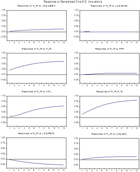

Figure-3. Response on DI future given shocks in variables.

Based on the analysis of the shock trajectories, it can be seen that the DI future responds positively and intensely to inflation shocks, as well as to shocks in the variable itself and in the spot interest rate. The response to shocks in economic activity is positive, but less intense than the aforementioned shocks analyzed, a pattern similar to that observed in the shocks that occurred in the public indebtedness variable. Finally, the DI future response is positive to shocks in the US interest rate and shocks in the country risk have no effect on the future interest rate.

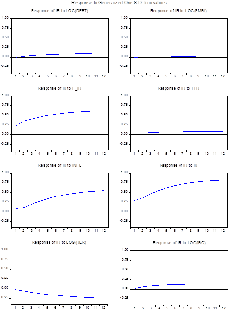
Figure-4 . Response on the Selic rate given shocks on variables.

In general, the responses to Selic rate shocks Figure 4 are similar to those seen in Figure 3. The Selic rate responds positively and intensely to shocks on inflation, on the rate itself and on the future interest rate. Concerning shocks on the inflation rate, there are similarities to the results found in Prado and da Silva (2017) and Segura-Ubiergo (2012), which reinforces the issue of the sensitivity of the monetary authority to price level fluctuations. The response to economic activity shocks is also positive, with Prado and da Silva (2017) finding a similar result when testing output gap shocks. The FIR signifies that there is a positive response, in the same direction and dissipating over time, of the Selic rate to shocks in the US interest rate, according to results obtained by Segura-Ubiergo (2012) and Barbosa et al. (2016).

The spot interest rate responses to shocks in public indebtedness are positive, as anticipated by Franco (2011), Segura-Ubiergo (2012) and Gottlieb (2013). The response to shocks in country risk is largely neutral, unlike in Barbosa et al. (2016), and the response to shocks in the real exchange rate contrasts the expected direction, unlike in Prado and da Silva (2017), who identified practically no effect on responses to shocks in short-term exchange rate fluctuations.

In addition to the results obtained by the Impulse Response Functions, it is possible to deepen the analysis with the application of statistical precedence tests, known as Granger causality. Causality, according to Granger, means that if one variable X causes another variable Y, then X can be considered a useful predictor of Y, as long as it precedes it in time. The Granger causality test consists of testing the hypothesis that the coefficients of the model variables are equal to zero using the F statistic. In this test, the null hypothesis (H0) defines that the variable X does not present causality in the Granger test in relation to variable Y, versus the alternative hypothesis that stipulates the opposite. H0 is not rejected when the p-value is > 0.05. The isolated test does not guarantee causality or non-causality between the variables under study, but it works as a check of statistical precedence, that is, it allows us to identify how much of the present value of Y can be explained by past values ​​of itself and then check whether adding lagged values ​​of X can improve the explanation.

The results of the Granger tests applied in this study are shown in Tables 4 and 5 and were obtained using the GRETL software. Bearing in mind the stationarity of the series, the lag tests were performed based on the available selection criteria of AIC, SC and Hannan-Quinn (HQ) in order to discover the ideal number of lags. Based on the selected optimal lag numbers, VAR models were estimated for each pair of variables, with the variables in first difference, with the exception of the US interest rate, which was already stationary in level.

Variables		Lags	F-value	p- value	Significance
FFR	Granger non-causality	3	0.3246	0.8075
F-IR	Granger non-causality	4	7.7168	0.0000	***
LDEBT	Granger non-causality	4	2.7595	0.0301	**
LEMBI	Granger non-causality	4	1.2306	0.3006
LIBC	Granger non-causality	3	5.1785	0.0020	***
INFL	Granger non-causality	3	0.8926	0.4466
LRER	Granger non-causality	3	3.6398	0.0143	**

Note: **rejection to the null hypothesis of no causality at 5% level of significance.***rejection to the null hypothesis of no causality at 1% level of significance.

From Table 4, it is not possible to reject the null hypothesis that the US interest rate, country risk and inflation variables precede the Selic rate in the period under analysis. Unlike the causality test in question, both Prado and da Silva (2017) and Segura-Ubiergo (2012) reinforce the sensitivity of the monetary authority to price level fluctuations. The statistical non-precedence between the US interest rate and the Selic rate also opposes the findings of Segura-Ubiergo (2012) and Barbosa et al. (2016). There is precedence of the economic activity variable for the Selic rate with a significance level of 1%, as found in Prado and da Silva (2017), which denotes a possible concern of the monetary authority in relation to the effects of its decisions on the level of economic activity.

The test suggests the existence of statistical precedence between the real exchange rate and the Selic rate with a 5% significance level. However, the results of Prado and da Silva (2017) for this relationship indicate that the real exchange rate is not important in the conduct of economic policy. The test indicates precedence at the 5% significance level of the public debt variable as a proportion of GDP to the Selic rate, as anticipated by Franco (2011), Segura-Ubiergo (2012), (Gottlieb, 2013) and Prado and da Silva (2017). This result is compatible with the deteriorating fiscal policy scenario, with signs of inconsistency in the performance of economic policy makers in relation to monetary and fiscal policies, with monetary policy being determined without intertemporal budget balance and resulting in a situation of fiscal dominance.

Variables		Lags	F-value	p-value	Significance
FFR	Granger non-causality	2	0.1308	0.8775
IR	Granger non-causality	4	9.5597	0.0000	***
LDEBT	Granger non-causality	2	0.4875	0.6915
LEMBI	Granger non-causality	2	0.0314	0.9925
LIBC	Granger non-causality	3	3.9319	0.0005	***
INFL	Granger non-causality	4	1.9116	0.1303
LRER	Granger non-causality	2	2.2882	0.0810	*

Notes: *rejection of the null hypothesis at 10% of significance level.***rejection of the null hypothesis at 1% of significance level.

In Table 5, the causality test indicates precedence between the Selic rate and the future interest rate at the 1% level of significance. On the other hand, the hypothesis that inflation shocks impact future interest rates is rejected, despite the movement observed previously in the FIR. There is also no evidence of statistical precedence involving country risk, public indebtedness or the US interest rate.

It is noteworthy that the Granger causality tests were complementary to the analysis carried out through the FIRs. Granger's causality test is a test of statistical precedence and not causality in the strictest sense of the term. Thus, if any variable did not show causality in the Granger sense, there is no invalidation of the estimated FIR. In this sense, the Granger causality test is a reinforcement of the analyses resulting from the VEC model. In addition, it is unequivocal to state that a prolonged period of international interest rates close to zero is unprecedented in the evolution of financial markets, which may also have affected the relationship of shocks and precedence between the variables analyzed in the study.

6. Final Considerations

This study aimed to evaluate the determinants of spot and future interest rates in Brazil between 2007 and 2019. Based on the econometric methodology used, the results indicate that both the Selic rate and the future-DI are influenced by fluctuations in the inflation, the level of economic activity and the US interest rates, in addition to being subject to the lagged effects of the variables themselves.

According to the FIRs, the effects of inflation shocks on interest rates are intensely observed and corroborate the conclusions of Prado and da Silva (2017) and Segura-Ubiergo (2012), denoting the sensitivity of the monetary authority to price level fluctuations. The effects of shocks in the level of economic activity on interest rates present the expected behavior, as observed in Prado and da Silva (2017), but less intensely than that seen for inflation.

Unlike the initial expectation, there is no correspondence between the real exchange rate, FIRs and the statistical precedence detected in the causality tests. The series graphs reveal devaluation behavior by the real exchange rate concomitant with a downward trend in interest rates. When observing the behavior of the real exchange rate from 2011 to 2019, there is a trajectory of exchange rate devaluation. The results of the FIRs to shocks in the real exchange rate were contrary to our expectations, likely due to the exceptional liquidity conditions prevailing in the period analyzed and to the fact that the real exchange rate is influenced, in addition, by the behavior of prices in the main trading partners of Brazil. Under normal conditions, it would be expected that the devalued real exchange rate would cause an increase in the prices of so-called tradables, which in turn would result in increased inflation and the need to raise the interest rate, in order to contain the inflationary effect.

Although causality tests have not shown statistical precedence between US and Brazilian interest rates, the FIRs indicate a direct relationship between these rates. When there is a shock in the North American interest rate, there is an increase in Brazilian interest rates; the opposite also applies. The trajectory of reduction observed in domestic rates is related to the fall and maintenance of the basic interest rate in the US at low levels for long periods of time.

The results indicated by the FIRs and the causality tests between the spot and forward rate deserve additional consideration. In both cases, there is a direct relationship between shocks and statistical precedence. Silva and Holland (2013) tested the causality and dependence of the interest rate in relation to the DI futures and show that the “bid-ask spread” of the DI futures market causes, in Granger's sense, the “bid-ask spread” of government bonds, which is a proxy for the spot interest rate. However, they suggest caution, as they remind the literature that future DI curves, used as references for the pricing of public bonds, constitute a peculiarity in the process of the formation of fixed interest rates in Brazil.

Regarding the limitations of this study, it is worth mentioning that it is not possible to assess the effects of variables that are difficult to measure or considered determinants of high Brazilian interest rates, such as the history of defaults and jurisdictional uncertainties related to the weaknesses of property rights and respect for contracts. The issue of the public debt burden has not been proven. Given the existence of competition between the public and private sectors for the resources needed for financing, it is intuitively expected that there will be an increase in interest rates as the growth of public debt in relation to GDP is observed, especially between 2016 and 2019.

As a suggestion for future work, given the context of exceptional liquidity conditions caused by the 2008 financial crisis, a window of opportunity is opened for studies that seek to prove the relationship between Brazilian interest rates and the US base rate. This is because the impulse response functions showed a direct relationship and in the same direction in the tests performed between them, but the Granger causality test did not show the expected statistical precedence, which leaves gaps for further studies on the relationship between the domestic interest market and its international counterpart.

References

Barbosa-Filho, N. H. (2008). Inflation targeting in Brazil: 1999-2006. International Review of Applied Economics, 22(2), 187-200.

Barbosa, F. d. H. (2006). The contagion effect of public debt on monetary policy: The Brazilian experience. Brazilian Journal of Political Economy, 26(2), 231-238. Available at: https://doi.org/10.1590/s0101-31572006000200004.

Barbosa, F. H. (2004). Interest rate inertia in monetary policy. Journal of Economics, 30(2). Available at: https://doi.org/10.5380/re.v30i2.2016.

Barbosa, F. H., Camêlo, F. D., & João, I. C. A. (2016). Natural interest rate and Taylor's rule in Brazil: 2003-2015. Brazilian Journal of Economics, 70(4), 399-417.

Biage, M. (2008). Country risk, capital flows and interest rate determination in Brazil: An analysis of impacts through the VEC methodology. Economy, 9(1), 63-113.

Blanco, F., & Holanda, F. (2010). Brazil: Resilience in the face of the global crisis. In  Nabli, M. K. (ed.) The Great Recession and Developing Countries (pp. 91-154). Washington: The World Bank.

Franco, G. H. B. (2011). Why are interest rates so high, and the path to normalcy. CLP Papers, São Paulo, Brazil, 6, 21-57.

Gottlieb, J. W. F. (2013). Estimates and determinants of the neutral real interest rate in Brazil. 2013. Master's Thesis, PUC-Rio, Rio de Janeiro.  

Johansen, S. (1991). Estimation and hypothesis testing of cointegration vectors in Gaussian vector autoregressive models. Econometrica: Journal of the Econometric Society, 59(6), 1551-1580. Available at: https://doi.org/10.2307/2938278.

Kindleberger, C. P., & Liber, Z. M. (2013). Panics and crises (pp. 609). São Paulo: Saraiva.

Lütkepohl, H. (1991). Introduction to multiple time series analysis (pp. 545). New York: Springer-Verlag.

Minella, A. (2001). Monetary policy and inflation in Brazil (1975-2000): A VAR estimation (pp. 33). Brasília, DF: Central Bank of Brazil, WorkingPaper Series.

Oliveira, F. N., & Ramos, L. O. (2011). Unanticipated monetary policy shocks and the term structure of interest rates in Brazil. Research and Economic Planning, Rio de Janeiro, 41(3), 433-470.

Oreiro, J., Paula, L., Silva, G., & Ono, F. (2006). Macroeconomic determinants of bank spread in Brazil: theory and recent evidence. Applied Economy, São Paulo, 10(4), 609-634.

Pessôa, S. (2013). Process of interest rate formation in Brazil: 1997-2012. Economy & Technology Magazine, 9(1), 163-168.

Pinheiro, A., & Amin, M. (2005). Capital flows and macroeconomic components: analysis of interrelationships through the application of a model and autoregressive vectors (VAR). 33st National Meeting of Economy-Anpec, Natal, Brazil, 33, 1-20.

Prado, P. H. M., & da Silva, C. G. (2017). Monetary policy and inflation targeting regime in Brazil: an analysis of the 2004-2014 period. Journal of Development and Public Policies, 1(1), 17-33. Available at: https://doi.org/10.31061/redepp.v1n1.17-33.

Segura-Ubiergo, A. (2012). The puzzle of Brazil’s high interest rate. Working Paper. International Monetary Fund.

Silva, A. L. P., & Holland, M. (2013). Market liquidity, future DI curve and the interest rate on fixed rate government bonds: Evidences for Brazil. Paper presented at the 41st National Meeting of Economy-Anpec. Foz do Iguaçu, Brazil, 41. 1-20.

Tabak, B. M., & Andrade, S. C. (2003). Testing the expectations hypothesis in the Brazilian term structure of interest rates. Brazilian Review of Finance, 1(1), 19-43.

Vartanian, P. R., & Garbe, H. S. (2019). The Brazilian economic crisis during the period 2014-2016: Is there precedence of internal or external factors? Journal of International and Global Economic Studies, 12(1), 66-86.

Vartanian, P. R. (2010). Currency and exchange rate shocks under floating exchange rate regimes in Mercosur member countries: Are there signs of macroeconomic convergence? EconomiA Magazine, 11(2), 435-464.