Social Expenditure and Competitiveness: Is there any Link? 

 

Emmanouil Karakostas

Department of International and European Studies, School of Economics, Business and International Studies, University of Piraeus, Piraeus, Greece.	Abstract Social policies form a part of every state’s basic economic policy. Many countries implement social policy measures to eradicate social conflicts. A key element of the design of any social measure is its financing. The main sources of financing for social benefits are fiscal policies and borrowing. Social expenditure is a key measure of a state's social policy. Although the exercise of social measures often significantly though indirectly benefits the society of a country, the basic assumption is that it places a certain direct burden on the country’s economy. Research says that social spending helps economic growth. The question is this: to what extent is social spending related to a state’s productivity? This question is critical for one reason in particular. Although social expenditure may be related to inflationary pressures or a slowdown in economic functioning, it may also help long-term economic functioning by stimulating productivity. The macroeconomic degree of productivity is important because the productivity of a state increases its competitiveness. This study will show whether social spending helps improve competitiveness. The methodology applied is ordinary least squares (OLS) multiple regression analysis.
Licensed: This work is licensed under a Creative Commons Attribution 4.0 License.
Keywords: Competitiveness OLS Productivity Social spending. JEL Classification: E60; H30; C10.
Received: 5 January 2022 Revised: 10 February 2022 Accepted: 25 February 2022 Published: 8 March 2022

Funding: This study received no specific financial support.

Competing Interests:The author declares that there are no conflicts of interests regarding the publication of this paper.

1. Introduction

Social spending is an important part of economic policy, although academics have voiced differing views on the consequences of social spending (Nembot, Melachio, & Kos, 2021). Keynesian theory, for instance, states that spending on public goods and services stimulates aggregate demand and economic growth. In contrast, neoclassical theory takes a more negative view because the public expenditure may bring about a decrease in private investment. Furthermore, the theory of endogenous development states that the key issue is the source of government funding because the source determines the outcome. Nonetheless, all agree that social spending affects the economy.

The study of the role of social spending has been mainly focused on economic growth. A key point of economic growth is productivity, which can be regarded as the cornerstone of a country's competitiveness (Alcalá & Ciccone, 2004; Choudhri & Schembri, 1999; Farole, Reis, & Swarnim, 2010; Kunst & Marin, 1989) . The current study aims to show whether social spending can have any effect on competitiveness through productivity. To achieve this aim, the paper will analyze two (2) countries: Switzerland and Germany.

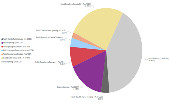
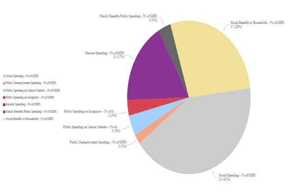
First, the average social expenditures of the concerned countries for the period 1995-2015 are presented. Figure 1 shows the average social expenditure for Switzerland for the above-mentioned period, while Figure 2 shows the average social expenditure for Germany.

It can be observed that the two countries follow a similar pattern. In both countries, the rate of social spending is highest, followed by the social benefits to households. Pension spending comes in third place. The question is whether this social expenditure affects competitiveness through productivity, which is what this study aims to clarify through the use of ordinary least squares (OLS) linear regression analysis.

The remainder of this paper is organized as follows: the second section provides a review of the relevant literature. The third section describes the methodology. The fourth section provides the results of the linear regression, and the final section concludes.

2. Review of the Literature

The literature on the topic is vast; this section, therefore, provides only a brief outline. The relationship between the reduction of income inequality and GDP growth has been the subject of many studies; research such as that of Benabou (2000); Okun (1975); Arjona, Ladaique, and Pearson (2003); Forbes (2000) and Ortega-Díaz (2006) has shown a positive relationship between the reduction of income inequality and GDP growth. Scholars such as Persson and Tabellini (1994); Alesina and Rodrik (1994); Easterly (2007); Perotti (1996); Berg, Ostry, Tsangarides, and Yakhshilikov (2018); Dabla-Norris, Kochhar, Suphaphiphat, Ricka, and Tsounta (2015) and Ostry, Berg, and Tsangarides (2014) have also investigated this relationship and report a negative effect. Surveys such as Baldacci, Clements, Gupta, and Cui (2008);  Singh (1996); Bakija, Kenworthy, Lindert, and Madrick (2016); Atkinson (1995); Berg et al. (2018) and Cingano (2014) have investigated the relationship between social spending and economic growth with varying results. Studies including Krueger and Pischke (1992); Krueger and Meyer (2002); French and Song (2014) and Rust and Phelan (1997) have explored the effect of social spending on labor supply.

More specifically, research such as Kim and Moody (1992); McGuire, Parkin, Hughes, and Gerard (1993); Musgrove (1996); Pritchett (1996); Filmer and Pritchett (1997); Filmer, Hammer, and Pritchett (1998); Bloom and Canning (2003) and Gyimah-Brempong and Wilson (2004) have reported on the effects of health expenditure. Studies such as Nijkamp and Poot (2004); Kocherlakota and Yi (1997); Noss (1991); Mingat and Tan (1998) and Flug, Spilimbergo, and Wachtenheim (1998) have reported the effects of education spending. Studies such as Anand and Ravallion (1993); Psacharopoulos (1994); Bidani and Ravallion (1997) and Psacharopoulos and Patrinos (2002) mention the role of social spending. Studies such as Mauro (1998) and Rajkumar and Swaroop (2002) mention the role management plays in the effectiveness of social spending. The next section describes the methodology of the current study.

3. Methodology and Data

This study investigates the relationship between social expenditure and productivity. The indicator “GPD per hour worked” is used as a measure of productivity (OECD, 2016). The categories of social expenditure included as independent variables are the percentages of GDP dedicated to “Social spending”, “Pension spending”, “Public unemployment spending”, “Family benefits public spending”, “Social benefits to households”, “Public spending on incapacity”, and “Public spending on labor markets”. The dependent variable is “GPD per hour worked”.

The database for this study is the OECD.¹ The period is 1995-2015. The period and the countries under investigation have been chosen primarily due to the availability of data. Moreover, the time period has been chosen because it represents a complete time frame of twenty years. The study uses traditional multiple regression analysis,² specifically the ordinary least squares (OLS) technique (Hutcheson, 2011).

 Table 1 shows the dependent variable and explanatory variables for Germany, and Table 2 shows the dependent variable and explanatory variables for Switzerland.

The study constructs the estimated multiple-regression model to test the above-mentioned hypotheses as follows:

where GPDpWt stands for GPD per hour worked (Total, 2015=10), β0 stands for the constant amount or the intercept, β1-β7 are coefficients of the explanatory variables, SocSpt stands for Social spending (%), PenSpt stands for Pension spending (%), PubUnSpt stands for Public unemployment spending (%), FamBPSpt stands for Family benefits public spending (%), SocBenHt: stands for Social benefits to households (%), PubSpInt: stands for Public spending on incapacity (%), PubSpLMt stands for Public spending on labor markets (%), e is the error term, t represents the year within the period 1995-2015, and i stands for the country.

The next section presents the results of linear regression.

Years	GDP per hour worked	Social Spending*	Pension Spending*	Public Unemployment Spending*	Family Benefits Public Spending*	Social Benefits to Households*	Public Spending on Incapacity*	Public Spending on Labor Markets*
1995	79.8	25.2	10.3	1.5	2.0	17.2	2.2	3.4
1996	81.2	25.8	10.5	1.6	1.9	17.9	2.3	3.6
1997	83.2	25.4	10.6	1.5	2.0	18.0	2.1	3.5
1998	84.0	25.3	10.7	1.4	2.0	17.7	2.1	3.3
1999	85.0	25.5	10.7	1.3	2.0	17.9	2.1	3.3
2000	87.1	25.4	10.8	1.3	2.0	17.5	2.1	3.0
2001	89.3	25.4	10.9	1.3	2.0	17.6	2.1	3.0
2002	90.1	26.1	11.1	1.4	2.0	18.1	2.1	3.3
2003	90.8	26.6	11.3	1.6	2.0	18.5	2.0	3.3
2004	91.6	26.0	11.2	1.7	2.0	18.1	2.0	3.3
2005	93.0	26.3	11.1	1.8	2.0	18.0	1.9	3.0
2006	94.5	25.1	10.7	1.6	1.7	17.1	1.8	2.5
2007	95.7	24.2	10.3	1.3	1.8	16.0	1.7	2.0
2008	95.7	24.3	10.3	1.2	1.9	15.9	1.8	1.9
2009	92.8	26.8	11.0	1.6	2.1	17.4	2.0	2.4
2010	94.9	26.0	10.7	1.4	2.1	16.7	1.9	2.1
2011	97.4	24.7	10.2	1.1	2.1	15.7	1.9	1.7
2012	98.0	24.6	10.2	1.0	2.1	15.6	1.9	1.6
2013	98.5	24.8	10.1	1.0	2.2	15.6	2.0	1.6
2014	99.5	24.7	10.0	0.9	2.2	15.4	2.0	1.5
2015	100.0	25.0	10.1	0.9	2.2	15.5	2.0	1.5

Source: OECD (2021b), OECD (2021c)*

Years	GDP per hour worked	Social Spending*	Pension Spending*	Public Unemployment Spending*	Family Benefits Public Spending*	Social Benefits to Households*	Public Spending on Incapacity*	Public Spending on Labor Markets*
1995	78.9	14.8	6.1	1.0	1.3	9.5	2.9	1.4
1996	80.6	15.1	6.1	1.1	1.3	10.0	2.9	1.6
1997	83.0	15.5	6.2	1.2	1.3	10.3	2.9	1.9
1998	84.0	15.5	6.2	1.0	1.4	9.9	2.9	1.7
1999	83.7	15.3	6.3	0.7	1.4	9.8	3.0	1.4
2000	86.4	14.4	6.0	0.5	1.4	9.1	2.9	1.0
2001	88.4	14.8	6.2	0.4	1.4	9.3	3.0	0.9
2002	88.9	15.7	6.2	0.7	1.5	9.8	3.3	1.2
2003	88.5	16.4	6.4	1.0	1.5	10.3	3.2	1.6
2004	89.1	16.3	6.2	1.0	1.4	10.2	3.2	1.6
2005	91.3	16.1	6.2	0.9	1.4	10.1	3.2	1.5
2006	93.5	15.3	5.9	0.8	1.4	9.5	3.2	1.2
2007	95.4	14.7	5.8	0.6	1.3	9.1	3.1	1.0
2008	96.3	14.4	5.7	0.5	1.4	8.8	2.8	0.9
2009	94.3	16.0	6.2	0.9	1.5	9.8	3.1	1.4
2010	97.8	15.7	6.1	0.9	1.5	9.7	2.8	1.3
2011	97.3	15.6	6.2	0.6	1.5	9.6	2.9	1.0
2012	97.7	15.9	6.3	0.6	1.5	9.6	2.8	1.1
2013	99.6	16.2	6.4	0.7	1.5	9.8	2.9	1.1
2014	100.7	16.1	6.4	0.7	1.6	9.8	2.7	1.1
2015	100.0	16.6	6.5	0.8	1.8	9.9	2.7	1.2

Source: OECD (2021b), OECD (2021c)*

4. Results

In this section, the results of the linear regression are presented. Table 3 shows the results of linear regression.

Dependent Variable:
	GDPpWt (Germany)	GDPpWt (Switzerland)
SocSpt	-6.525 (-14.565, 1516)	16.356*** (11.468, 21.243)
PenSpt	16.150* (1.512, 30.788)	-32.750*** (-45.030, -20,469)
PuUnSpt	12.601 (-5.609, 30.810)	-15.674* (-30.055, -1.293)
FamBPSpt	5.411 (-9.891, 20.714)	-11.533 (-31.102, 7.996)
SocBenHt	2.253 (-6.345, 10.851)	2.884 (-7.063, 12.832)
PubSpInt	24.407 (-14.695, 63.509)	-22.768*** (-30.660, -14.876)
PubSpLMt	-17.635** (-29.781, -5.489)	-10.682* (-21.489, 0.125)
e	0.396 (-1.020, 1.813)	-0.212 (-1.046, 0.622)
Constant	15.201 (-47.033, 77.435)	124.774*** (90.597, 158.950)
Observations	21	21
R2	0.952	0.968
Adjusted R2	0.921	0.947
Residual Std. Error (df=12)	1.735	1.550
F Statistic (df=8; 12)	30.005***	45.669***

Note:  *p<0.1; **p<0.05; ***p<0.01.

The results of the linear regression prove the functionality of the model. The next section presents the conclusions of this study.

5. Conclusion

This study has examined whether a relationship exists between social spending and GDP per hour worked. Adjusted R2 is high, in both Germany and Switzerland. In the case of Switzerland, it is 0.94, while in the case of Germany, it is 0.92. This means that the model constructed in this study serves to explain the relationship between the independent variables and the largely dependent one. The greater the adjusted R2, the better the model fits the data. In the case of Germany, the variables SocSpt and PubSpLMt have a negative effect on the GDP per hour worked, whereas the remaining variables have a positive effect. In the case of Switzerland, the variables PenSpt, PubUnSpt, FamBPSpt, PubSpInt, and PubSpLMthave a negative effect on the GDP per hour worked, whereas the other variables have a positive effect.

Social expenditure is an integral part of the economic policies of each state. The analysis carried out in this study confirms that social expenditure affects productivity. If we consider productivity to be the backbone of competitiveness, then social expenditure indirectly affects a state’s competitiveness. Further research is required to develop a comprehensive analytical framework through which the selected variables can explain the phenomenon.

References

Alcalá, F., & Ciccone, A. (2004). Trade and productivity. The Quarterly Journal of Economics, 119(2), 613-646.

Alesina, A., & Rodrik, D. (1994). Distributive politics and economic growth. The Quarterly Journal of Economics, 109(2), 465-490.

Anand, S., & Ravallion, M. (1993). Human development in poor countries: On the role of private incomes and public services. Journal of Economic Perspectives, 7(1), 133-150.Available at: https://doi.org/10.1257/jep.7.1.133.

Anghelache, C., Anghel, M. G., Prodan, L., SACALA, C., & Popovici, M. (2014). Multiple linear regression model used in economic analyses. Romanian Statistical Review Supplement, 62(10), 120-127.

Arjona, R., Ladaique, M., & Pearson, M. (2003). Growth, inequality and social protection. Canadian Public Policy, University of Toronto Press, 29(s1), 119-140.

Atkinson, A. B. (1995). Is the Welfare State necessarily an obstacle to economic growth? European Economic Review, 39(3-4), 723-730.Available at: https://doi.org/10.1016/0014-2921(94)00079-f.

Bakija, J., Kenworthy, L., Lindert, P., & Madrick, J. (2016). How big should our government be? Berkeley, CA: University of California Press.

Baldacci, E., Clements, B., Gupta, S., & Cui, Q. (2008). Social spending, human capital, and growth in developing countries. World Development, 36(8), 1317-1341.Available at: https://doi.org/10.1016/j.worlddev.2007.08.003.

Benabou, R. (2000). Unequal societies: Income distribution and the social contract. American Economic Review, 90(1), 96-129.Available at: https://doi.org/10.1257/aer.90.1.96.

Berg, A., Ostry, J. D., Tsangarides, C. G., & Yakhshilikov, Y. (2018). Redistribution, inequality, and growth: New evidence. Journal of Economic Growth, 23(3), 259-305.Available at: https://doi.org/10.1007/s10887-017-9150-2.

Bidani, B., & Ravallion, M. (1997). Decomposing social indicators using distributional data. Journal of Econometrics, 77(1), 125-139.Available at: https://doi.org/10.1016/s0304-4076(95)01809-3.

Bloom, D., & Canning, D. (2003). The health and poverty of nations: From theory to practice. Journal of Human Development, 4(1), 47-71.Available at: https://doi.org/10.1080/1464988032000051487.

Choudhri, E. U., & Schembri, L. L. (1999). Productivity performance and international  competitiveness: A new test of an old theory. Paper presented at the Carleton Economic Papers 99-02,  Carleton University, Department of Economics, revised May 2002.

Cingano, F. (2014). Trends in income inequality and its impact on economic growth. OECD Social, Employment and Migration Working Paper, No. 163, Paris, Organisation for Economic Co-operation and Development.

Dabla-Norris, E., Kochhar, K., Suphaphiphat, N., Ricka, F., & Tsounta, E. (2015). Causes and consequences of income inequality: A global perspective. IMF Staff Discussion Note, 15/13. . Washington, D.C: International Monetary Fund.

Easterly, W. (2007). Inequality does cause underdevelopment: Insights from a new instrument. Journal of Development Economics, 84(2), 755-776.Available at: https://doi.org/10.1016/j.jdeveco.2006.11.002.

Farole, T., Reis, J. G., & Swarnim, W. (2010). Analyzing trade competitiveness: A diagnostics approach. Policy Research Working Paper No 5329, International Trade Department, The World Bank, June 2010.

Filmer, D., & Pritchett, L. (1997). Child mortality and public spending on health: How much does money matter? World Bank Policy Research Working Paper No. 1864 (Washington: World Bank).

Filmer, D., Hammer, J., & Pritchett, L. (1998). Health policy in poor countries: Weak Links in the Chain. World Bank Policy Research Working Paper No. 1874, (Washington: World Bank).

Flug, K., Spilimbergo, A., & Wachtenheim, E. (1998). Investment in education: Do economic volatility and credit constraints matter? Journal of Development Economics, 55(2), 465-481.

Forbes, K. J. (2000). A reassessment of the relationship between inequality and growth. American Economic Review, 90(4), 869-887.Available at: https://doi.org/10.1257/aer.90.4.869.

French, E., & Song, J. (2014). The effect of disability insurance receipt on labor supply. American Economic Journal: Economic Policy, 6(2), 291-337.

Gyimah-Brempong, K., & Wilson, M. (2004). Health human capital and economic growth in Sub-Saharan African and OECD countries. The Quarterly Review of Economics and Finance, 44(2), 296-320.Available at: https://doi.org/10.1016/j.qref.2003.07.002.

Hutcheson, G. D. (2011). Ordinary least-squares regression. In: Moutinho, L. and Hutcheson, G.D., The SAGE Dictionary of Quantitative Management Research (pp. 224-228). Thousand Oaks: Sage Publications.

Kim, K., & Moody, P. M. (1992). https://doi.org/10.1016/0277-9536(92)90253-m. Social Science & Medicine, 34(8), 837-842.Available at: https://doi.org/10.1016/0277-9536(92)90253-m.

Kocherlakota, N. R., & Yi, K.-M. (1997). Is there endogenous long-run growth? Evidence from the United States and the United Kingdom. Journal of Money, Credit, and Banking, 29(2), 235-262.Available at: https://doi.org/10.2307/2953677.

Krueger, A. B., & Pischke, J.-S. (1992). The effect of social security on labor supply: A cohort analysis of the notch generation. Journal of Labor Economics, 10(4), 412-437.Available at: https://doi.org/10.1086/298294.

Krueger, A. B., & Meyer, B. D. (2002). Labor supply effects of social insurance. Handbook of Public Economics, 4, 2327-2392.Available at: https://doi.org/10.1016/s1573-4420(02)80012-x.

Kunst, R. M., & Marin, D. (1989). On exports and productivity: A causal analysis. The Review of Economics and Statistics, 71(4), 699-703.Available at: https://doi.org/10.2307/1928115.

Mauro, P. (1998). Corruption and the composition of government expenditure. Journal of Public Economics, 69(2), 263-279.Available at: https://doi.org/10.1016/s0047-2727(98)00025-5.

McGuire, A., Parkin, D., Hughes, D., & Gerard, K. (1993). Econometric analyses of national health expenditures: Can positive economics help to answer normative questions? Health Economics, 2(2), 113-126.Available at: https://doi.org/10.1016/s0047-2727(98)00025-5.

Mingat, A., & Tan, J. P. (1998). The mechanics of progress in education: Evidence from cross-country data. Policy Research Working Paper No. 2015 (Washington: World Bank).

Musgrove, P. (1996). Public and private roles in health: Theory and financing patterns. World Bank Discussion Paper No. 339 (Washington: World Bank).

Nembot, N. L., Melachio, T. A., & Kos, A. M. A. (2021). Effects of public expenditure on economic growth in the CEMAC Subregion: A comparative analysis between the fragile and non-fragile states. AERC Working Paper FW-006, African Economic Research Consortium, Nairobi, May 2021.

Nijkamp, P., & Poot, J. (2004). Meta-analysis of the effect of fiscal policies on long-run growth. European Journal of Political Economy, 20(1), 91-124.Available at: https://doi.org/10.1016/j.ejpoleco.2003.10.001.

---

Footnotes: