The Effects of Annual GDP Growth on Consumption Spending: Evidence from West African Countries 

 

Ismaila Y Jammeh

Department of Economics, Management and Industrial Engineering, University of Aveiro, Aveiro, Portugal.	Abstract This study examines the effect of annual growth in the gross domestic product (GDP) on consumption spending in West African Countries from the period 2005 to 2020. Consumption has been a fundamental driver of economic growth, and insufficient consumption spending will lure firms to lay off workers which can lead to short-run fluctuation in the economy. The study employed a dynamic panel model with a set of estimation strategies such as fixed and random effect, Anderson and Hsiao estimation method, difference and System-Generalized Methods of Moment and Least Square Dummy Variable estimation methods to correctly assess how annual growth in the gross domestic product (GDP) affects consumption spending in these countries including additional variables such as Lag consumption spending, foreign direct investment, consumer prices as a measure of inflation and a vector of control such as capital formation and annual population growth. The study found that annual GDP growth and Foreign direct investment have a significant impact on increasing consumption spending thus annual GDP growth is the most crucial factor for increasing consumption spending in these countries. Moreover, lagged consumption spending is also found to have a negative significant effect in reducing current consumption spending while gross capital formation and annual population growth are found to have an insignificant effect in reducing consumption spending in all the estimates except in the Anderson and Hsiao estimation method which shows a positive relationship with consumption spending.
Licensed: This work is licensed under a Creative Commons Attribution 4.0 License.
Keywords: GDP growth Consumer spending Panel data Generalized method of moment Least square dummy variable.
Received: 4 July 2022 Revised: 8 August 2022 Accepted: 24 August 2022 Published: 12 September 2022

Funding: This study received no specific financial support.

Competing Interests:The author declares that there are no conflicts of interests regarding the publication of this paper.

1. Introduction

At the start of the Covid-19 pandemic which put every economic and non-economic activity at a halt, people were in a panic, some engage in panic buying, thinking that the pandemic will never be over while others were thinking that when the government lockdown the economy, they will not be able to consume the same level they usually enjoyed before the pandemic.

During this unprecedented time, we became more upset, perplexed and hopeless when we lost jobs that were so dared to us that we’ve never thought of losing, post us a serious question, why are firms laying-off workers during this hard time, and why are government not taking any action. They probably did what they could do best when many governments around the world introduced stimulus packages that gave households cash bonuses to continue enjoying the goods and services they always enjoyed before the pandemic. This explains why is important to know how economics works and why government give cash bonuses when people are losing their jobs in a crisis situation is fundamentally important in restoring hope and confidence in the economy and crucial as a determinant of economic growth (Mankiw, 2019).

Consumption spending has been a fundamental driver of economic growth, an increase in consumption expenditure by households and the government boost aggregate demand in the economy which also makes it profitable for firms to increase their production level by employing more workers and this implies more taxable income for the government. Understanding household consumption spending seems to be a micro question but answering this kind of question significantly depends on the macroeconomic conditions (Mankiw, 2019).

The Keynesian consumption theory (Mankiw, 2019) saw consumption as a function of disposable income, the more the economy develops means the central government will have more revenue for investment and create more job opportunities for its people and thus more jobs mean people will have more income to spend in the economy and this can also depend on government policies that will encourage more spending in the economy such as promoting price stability, reduction in income tax which increases consumers disposable income. Giving this interrelation s very optimistic that short-run fluctuation in the economic is cause by the lack of aggregate demand (cited in Snowdon & Vane, 2005) which also convinced firms that they have to lay-off workers giving that what they have been producing has not been demanded by the consumer while paying them wages or salaries. The more firms produce goods and services also means these firms will employed more workers who are the households and paying them higher wages or salaries and this also implies households will have more income to spend in the consumption of goods and services produced and firm will have incentives to increase their production, employing more workers and paying higher wages or salaries to these households which is beneficiary for the economy at an aggregate level by increasing employment and generating revenue to the government to spend on other infrastructural projects (Radulescu, Serbanescu, & Sinisi, 2019).

Therefore, giving the important of consumption spending on macroeconomic performances, this study examines how annual GDP growth will impact consumption spending in the West African Countries, which has received less academic attending with the existence of scarce studies on this issue.

2. Literature Reviews

The main purpose of this paper is to empirically examine the impact of annual GDP growth on consumption spending which will help to understand how government policies will affect consumer behaviors and thus provide more information in measuring the persistence of poverty and inequality in these countries. In doing so, the study will also examine how other macroeconomic variables such as foreign direct investment, gross capital formation, population growth and consumer prices affect consumption spending in these countries. Consumption will directly measure the household’s well-being and even if income changes with the rate of inflation rate, by only measuring the amount earned will be mis-leading in analyzing the well-fare of the consumer but with the amount consumed by a consumer, will give us more information about the consumer well-fare and we can observe if the well-fare of the consumer improved or not.

Several researchers have studied how annual GDP growth can affect consumption spending in most developed and emerging economies (Alper, 2018; Diacon & Maha, 2015; Radulescu et al., 2019) but little effort has been done to understand how annual GDP growth will stimulate consumption spending in this region which will enable us to understand and analysis how consumers will respond to a change in government policies in these countries. Keynes (1936) from his study of business cycles, believed that consumption spending depends on disposable income, if income of individuals increases will lead them to increase their consumption spending (cited in Mankiw, 2019). But in aggregate term, public consumption spending will increase if gross domestic product increases which measures national income. The more revenue generated by a country will translate to large government investment which will create more jobs and pay higher wages to its people to increase their consumption spending giving that there are stable prices and low taxation. National income also depends on the level of individual consumption spending, the more people spend in the economy, the more firms will increase their production level. Keynes (1936) has also shown in the Keynesian cross, that an increase in consumption has a multiplier effect on output, as planned expenditure increases, aggregate output will increase more than the increase in consumption spending. Therefore, short run economic fluctuation is due to lack of effective demand (cited in Snowdon & Vane, 2005).

Modigliani (1966) and Friedman (1957) in their Lifecycle and Permanent Income Hypothesis theories respectively also verified the validity of the Keynesian theory which they believed, if households will want to smoothen their consumption over time, then they will be engaging in forward looking behaviors, and their spending should not be based on current income but on the income, they expect to receive. They each used different approach to explained forward-looking behavior of consumers (Mankiw, 2019).

The later approach believes consumption depends on both wealth and income, if households always want to smoothen consumption over their lifetime, giving that savings can allow them to consume more during retirement when income is low by saving during their working periods, will choose to save more of their income so that they can be able to consume the same quality of goods and services consume before. While the Friedman (1957) approach believes peoples income to be the sum of transitory and permanent income. Transitory income is the unexpected income that individuals receive such as winning a lottery ticket, receiving a present on your birthday and so on. while the permanent income is the expected income that individual expect to receive during their working periods. He further argues that consumption spending is function of permanent income and transitory income determines savings of individuals (Romer, 2019).

In addition to Modigliani (1966) and Friedman (1957) theories, Hall (1978) in his Random Walk Hypothesis believes rational individuals will use all available information in forecasting their future consumption behaviors, therefore he further argues that if the Friedman theory is correct and individuals are rational and use all information available, then change in consumption will not be predictable overtime which means that households consumption changes as income change will follow a random walk (Mankiw, 2019; Romer, 2019).

Moreover, giving the different explanations of the consumption behaviors of households as sole determinant of production. Understanding consumption patterns of individual households is fundamental to comprehend economic fluctuation and predict how consumers will respond if policy changes. There have been also a body of research that used micro and macro data in several parts of the world to understand how household and government consumption can affect many macroeconomic variables and national income in particular.

Campbell. and Mankiw (1989) in their earlier findings by using aggregate data in the United States found that the rule of thumb by which consumption should change as income change is around 0.50. Campbell and Mankiw (1990) further replicated this study to investigate how consumption will response when income changes in different periods in the UK, Canada, France, Japan and Sweden and they also estimated the rule of thumb which they found match their earlier estimation and they concluded that change in consumption is not only on permanent income, if household current income increases, will increase their consumption level.

Lusardi (1996) further employed the Euler equation of first order conditions of consumer’s maximization problems to verify the Campbell and Mankiw estimation of the rule of thumb, which she also found, values close to the Campbell and Mankiw estimates to be the rule of thumb. She further argues that consumption is sensitive to predicted income changes therefore, random walk hypothesis which predicts that consumption cannot be predicted overtime do not hold.

In understanding the pattern of consumption spending during period of low income and period of large income, Sarmento, Marques, and Galan-Ladero (2019) investigated how consumption is affected during period of recession and recovery in Portugal in 2014 and 2018 recovery process using the snowball method to interview 11 consumers with 22 interviews and they found that, during recession in Portugal, there was an increasing social responsibility which leads to planned behaviors, households buy less and more frequently and buy more private labels while during recovery households tends to save more. Therefore, they concluded that during recession household’s consumption behavior and lifestyle changes and consumers are more concern about financial security.

Alper (2018) also studies the nexus between economic growth, consumption, investment, savings, unemployment and portfolio investment applying a panel data from 2005-2016 in Brazil, Russia, India, South Africa and Turkey. He found that increasing in consumption, savings and investment will increase economic growth in these countries while portfolio investment and unemployment were found to have insignificant effects. From his findings, if consumption increase by 1% will lead to an increase in economic growth by 0.41% in these countries.

Diacon and Maha (2015) employed a time series approach to study the relationship between consumption and GDP using a cross country analysis of 79 low, middle and high-income countries from 1980 to 2010 and found that there is a strong relationship between consumption and GDP in low and high-income countries while a weak relationship in middle-income countries during the period of studies.

Pollock (2009) uses a spectral analysis approach in the UK to study the relationship between consumption and income and found that fluctuation in consumption will have the same impact as the fluctuation in income.

Rafiy, Adam, Bachmid, and Saenong (2018) investigated how consumption spending and investment affect economic growth in Indonesia, using an autoregressive distributed lagged model (ARDL) model approach from 2003 to 2013.

The studies found that consumption have both short run and long run effect on economic growth, if consumption of household and government spending increases by 1% will cause an increase in economic growth by 1.88% while Handriyani, Sahyar, and Si (2018) studies the effects of household’s consumption spending, interest rate and investment on economic growth focusing on the Sumatera Utara region in Indonesia using simultaneous equation model. They found that consumptions of households in this region have a positive significant effect on economic growth, the more the household’s income, the more consumption will increase.

Spasojevic and Dukic (2018) study how consumption, foreign direct investment and domestic investment will affect economic growth in the Republic of Srpska from 2007 to 2016 which they found that consumption, domestic and foreign direct investment have a positive significant impact on GDP growth.

Radulescu et al. (2019) also uses a panel data approach in eight (8) Central and Eastern European countries from 2004-2017 to check how consumption and investment affect growth including additional control variables such as foreign direct investment, corruption perception index, share of corporate income tax, unemployment, net export, savings and government spending which they also found that if government spending increases will lead to increase in private consumption spending which has a positive effect on economic growth in the short run but in the long run this may not hold if people start to import more foreign goods in the domestic economic, thus, consumption lead growth holds in these countries. Their study also found a weak correlation between foreign direct investment and growth while a positive relationship between institutions and economic growth.

In Iran, Nikbin and Panahi (2016) applied an ARDL approach to co-integration to study the relationship between total private consumption on GDP growth, inflation and lagged of total private consumption from 1978 to 2012. They found that a percentage point change in private consumption will lead to 1.13% change in GDP growth and a negative correlation between inflation and total private consumption and they further argue that Consumption responds sluggishly to GDP growth in the short run than in the long run.

There has been difference choice of variables used in studying the relationship between consumption and GDP growth in many studies. This study is similar to the study of Nikbin and Panahi (2016) who used lagged total private consumption but different in estimation approach and other explanatory variables.

3. Methods

3.1. Model Specification

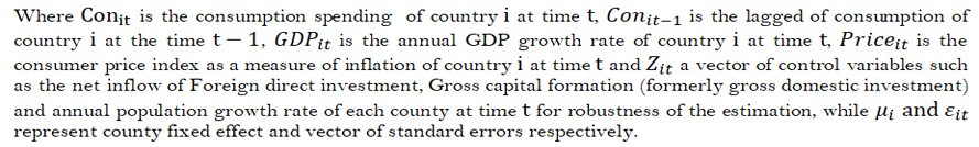
This study used a dynamic model panel model in examining the effects of annual GDP growth on consumption spending in these West African countries which can be econometrically represented as.

3.2. Data Source

The data used in assessing the effects of annual GDP growth on consumption spending in these countries are obtained from the World Bank Development indicators for a total of fourteen countries such as Benin, Burkina-Faso, Ivory-Coast, The Gambia, Ghana, Guinea, Guinea-Bissau, Mali, Mauritania, Niger, Nigeria, Senegal, Sierra-Leone and Togo.

Moreover, the remaining two West African Countries, Cape Verde and Liberia were excluded from the studies due to lack of sufficient data availability in these countries, excluding them in the studies will not affect the validity of the studies giving that the major contributors to the West African economy are included in the studies. Therefore, these fourteen (14) countries can help to examine how annual GDP growth affect consumption spending in these countries.

All the data used in this study are in annual frequencies covering a period of sixteen (16) years from 2005 to 2016.

Gross capital formation as a measure of physical capital and population growth has been a key factor in explaining neoclassical growth model of economic growth, including them in the model will help to account for their contributions to economic growth in these countries (Alper, 2018; Handriyani et al., 2018; Radulescu et al., 2019; Spasojevic & Dukic, 2018) all uses foreign direct investment and domestic investment in their studies on the relationship between consumption and GDP growth as a measure of income.

There is mixed relationship between consumption and income, income can determine individual consumption spending, the inverse is also true (Campbell & Mankiw, 1990; Lusardi, 1996) all used consumption as dependent variable to study its relationship with Income. Thus, it’s the main tenet of the Keynesian consumption theory and lagged consumption is used to capture how previous period consumption will affect current consumption spending, including this lagged consumption will also account for the factors that affect last period consumption.

In estimating the relationship between consumption spending and annual GDP growth in the West African Countries, the study employed a panel data approach to be able to capture unobserved heterogeneity in these countries. Hsiao (2007) explains the advantages of using panel data analysis, which he stated that, the use of panel data will help to overcome endogeneity problem which is because the strength of the estimation methods in controlling for the country fixed effect and the time series dimension and thus panel data analysis will provide efficiency in the estimation by providing more degree of freedom, more information and more sample variability to make an accurate inference about the estimated model. While Paleologou (2013) gives a problem, we might encounter when using panel data analysis. which he argues its ability to reduce efficiency if the time series dimension is small or considering subjects from different geographical region, social and economic development. Moreover, this is not an issue in this study since it focusses on countries in the same region and almost the same economic status, then the efficiency of this estimation will not be affected.

4. Pre-Estimation Analysis

Before empirically estimating the effect of annual GDP growth on consumption spending in these West African Countries, I performed a pre-estimation analysis to know the nature and distribution of the variables understudy. After performing the analysis, all the variables where found to be free from outliers and normally distributed which if not they may lead to heteroscedasticity and thus this can have serious consequences on the efficient of the estimates.

Furthermore, I also check the stationarity of the variables, using 5 lagged periods, which is crucial before making any analysis, knowing the stationarity of the variables will help to know if the statistical properties change over time or not. In performing the stationarity test, I performed Augmented Dickey-Fuller test to examine if there are unit roots in the variable which has a probability of large p-value, which show no evidence of non-stationarity in the variables during the period of consideration and the result are presented in Table 1.

Variables	Lags	Dickey-Fuller	p-value	Alternative hypothesis
Consumption Spending	5	-6.101	0.01	Stationary
GDP Growth	5	-4.839	0.01	Stationary
Foreign Direct Investment	5	-4.822	0.01	Stationary
Population Growth	5	-2.776	0.25	Stationary
Gross Capital Formation	5	-3.643	0.03	Stationary
Consumer Price	5	-2.693	0.285	Stationary

Moreover, I also performed a descriptive statistical analysis to fully observed the distribution of the data, which show a low consumption spending (4.33) on average in these countries and there hasn’t been much difference in these countries consumption spending and this is capture by the low standard deviation compared to the maximum amount spend on consumption. Giving the contribution of consumption spending on economic growth, the lack of consumption spending might be a result of the low average annual GDP growth during the period, but the average GDP growth slightly above the average consumption spending and there have been little difference in their economic growth rates.

When I checked the nature of foreign direct investment variables, I observed that there has been a low average rate of growth on this variable and not much difference in the growth rate in these countries, this can be the lack of good governance, political and economic stability in these countries which make foreign investors skeptical in investing in these countries. The average rate of annual population growth is very significant and almost the same in these countries while average rate of capital formation (formerly domestic investment) is also very significant in these countries and there is not much different in their domestic capital investment growth rates. Finally, the consumer prices are not very significant but there is a huge different in their increments in consumer prices. The differences in their consumer prices are very significant and the result of this descriptive statistics are shown Table 2.

Variables	Min	Mean	Variance	Std. Dev	Max
Consumption Spending	-16.3	4.33	35.83	5.99	39.03
GDP Growth	-20.6	4.52	14.11	3.76	20.72
Foreign Direct Investment	-11.2	3.74	20.41	4.52	32.3
Population Growth	2.04	2.76	0.17	0.41	3.91
Capital Formation	6.7	21.88	63.33	7.96	52.67
Consumer Price	-3.23	5.31	33.89	5.82	34.7

The study also conducted a Pearson correlation matrix on the variables of studies shown in the Table 3 below which measures the linear correlation between the variables. From the correlation matrix, it shows a significant positive correlation between consumption spending with annual GDP growth, FDI and gross capital formation, which is the total domestic investment while there’s a negative correlation with annual population growth and consumer prices.

Variables	Consumption Spending	GDP	FDI	Population	Capital Formation	Consumer Prices
Consumption	1	0.345	0.191	-0.002	0.038	-0.034
GDP	0.345	1	0.183	0.070	0.142	-0.004
FDI	0.191	0.183	1	-0.001	0.397	0.198
Population	-0.002	0.070	-0.001	1	0.222	-0.410
Capital Formation	0.038	0.142	0.397	0.222	1	-0.030
Consumer Prices	-0.034	-0.004	0.198	-0.410	-0.030	1

The positive correlation between annual GDP growth and consumption expenditure means they move in the same direction, an increase in annual GDP growth will likely cause consumption to increase in these countries which is true because an increase in income means consumers and government are more likely to spend on consumption and this conformed with other studies. Moreover, the correlation between inflow of foreign direct investment (FDI) is not very high as it does with annual GDP growth. While annual population growth and consumer price level are found to have a very small correlation. As shown in the correlation matrix, I can firmly confirm that the variables used in model is significant in estimating the effects of annual GDP growth on consumption spending in the West African Countries during the period of studies giving that none of the correlation between the variable reach the accepted threshold for the present of multicollinearity but this is just a simple correlation analysis, the result of the empirical estimation will help to determine the effects of these variables on consumption spending in these countries.

5. Results of Empirical Estimation

5.1 Pooled OLS, Fixed and Random effect estimation Method

Moreover, giving the different assumptions of the panel data estimator, I performed the Hausman test to identified if the model (1) specified above is a fixed effect or a random effect model.

Firstly, before identifying this, I performed Lagrange Multiplier Test - two-ways effects (Gourieroux, Holly, & Monfort, 1982) to check if there is significant two-ways effect, which report a p-value of 0.6007 indicating that there is insignificant two-ways effect in these countries. Now that we identified that, I also performed the Hausman test on the fixed effect model and random effect mode (time effect) which also reported p-value of 8.274e-05 (0.0557) supporting the null hypothesis that the heterogeneities present within these West African Countries are just random component. Meaning that these countries heterogeneities such as their government policies, culture or geography might not lead to different consumption spending, this is very true in the sense that these countries almost have the same standard of living, almost similar cultures, persistent of corruption in their governments, there are no unique policies that can lead them to differentiated consumption spending.

Furthermore, I also ran a Wooldridge's test for unobserved individual effects in panel model and this also support the null hypothesis with a p-value (0.0701) more than the significant level thus means there is no unobserved individual effect in the panel model. In addition, giving that these countries unobserved heterogeneity is random variation. Table 4 presents an empirical estimation of the pooled OLS; fixed effect and the two-ways random effect estimates but the analysis is based on the time random effect estimates.

Variables	Consumption
	Pooled-OLS	Fixed-Effect	Two-ways Effect	One-way
Effect
Lag Consumption	-0.47*** (0.06)	-0.49*** (0.06)	-0.48*** (0.06)	-0.47*** (0.06)
GDP Growth	0.73*** (0.10)	0.77*** (0.11)	0.74*** (0.10)	0.73*** (0.10)
Foreign Direct Investment	0.29*** (0.09)	0.28** (0.11)	0.27*** (0.10)	0.29*** (0.09)
Population Growth	-0.63 (0.98)	-5.28* (2.75)	-1.46 (1.42)	-0.63 (0.98)
Capital Formation	-0.07 (0.05)	-0.12 (0.08)	-0.08 (0.06)	-0.08 (0.06)
Consumer Prices	-0.09 (0.07)	-0.15 (0.11)	-0.11 (0.09)	-0.09 (0.07)
Constant	5.86** (2.84)		8.52** (4.15)	5.84** (2.83)
Observations	210	210	210	210
R2	0.34	0.35	0.34	0.34
Adjusted R2	0.32	0.29	0.32	0.32
F Statistic	17.41*** (df = 6; 203)	17.32*** (df = 6; 190)	105.22***	103.75***

Note: significant levels *p<0.1; **p<0.05; ***p<0.01;   standard errors in parenthesis ()

The empirical estimation reported a higher coefficient of determination than the accepted threshold which indicated that dynamic model is significant in explaining consumption spending in these countries and the rest due to errors and thus more support of this model, the F-Statistics also shows that all the variables included in the model are jointly significant in explaining consumption spending in the West African Countries during the period of studies.

Due to the Nickel biased that may arise on the lag dependent variable with the fixed and time effect estimation in the model (1), given the error term might correlate with the lag dependent variable.

The Aderson and Hsiao (1982) method will be able to eliminate the country specific fixed effect by taking the first difference of the model and used  or more lags as instrumental variable.

5.2. Anderson and Hsiao Estimation Method

In estimating the Anderson and Hsiao method below,

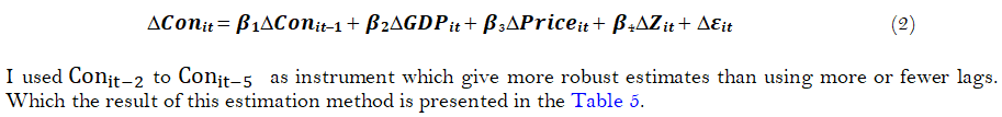
The low p-value also indicated that this estimation method is significant in assessing the impact of these variables on consumption spending in the West African Countries. During this period, these variable impacts have a 10% significant level in improving consumption spending in 2013 while a lead to a reduction in consumption spending in 2014. Moreover, about 50% of the change in consumption spending during the period of studies was explained by the change in these variables which is capture by the high R square which is more than the accepted threshold.

Instrumental variable estimation (Balestra-Varadharajan-Krishnakumar's transformation) Balanced Panel: n = 14, T = 11, N = 154 Residuals: Min.                1st Qu.         Median         3rd Qu.       Max. -25.232811   -2.460120      0.098116       3.287460     26.261196 Difference Consumption
Lag Difference in Consumption	-0.490*** (0.095)
Difference GDP Growth	0.795*** (0.286)
Difference Foreign direct Investment	0.030 (0.549)
Difference Population Growth	26.281 (21.488)
Difference Gross Capital	0.161 (0.376)
Difference Consumer Prices	-0.211 (0.476)
Year 2010	-1.469 (2.057)
Year 2011	1.126 (2.736)
Year 2012	-1.901 (2.212)
Year 2013	3.870* (1.983)
Year 2014	-3.843* (2.123)
Year 2015	1.683 (2.037)
Year 2016	-0.695 (1.877)
Year 2017	-0.225 (2.003)
Year 2018	0.495 (1.951)
Year 2019	-0.264 (1.968)
Year 2020	1.233 (2.323)
Observations             154           R2                               0.493             Adjusted R2               0.434            F Statistic                  64.111***   p-value:                      2.1699e-07       Chisq: 64.1109 on 17 DF

Note:  significant levels *p<0.1; ***p<0.01;  standard errors in parenthesis.

5.3. Generalized Method of Moments Estimation Method

The Generalized Method of Moment (GMM) estimation produces an efficient estimate due to its ability to provide all available moment conditions which are greater than the parameters. I estimated the dynamic consumption model using both one-step difference GMM and one-step system GMM. As argued by Arellano and Bond (1991) the failure of the Anderson and Hsia estimation method to use all available moment conditions may lead to inefficient estimates, which they proposed using the difference GMM estimator, which will be able to remove the countries unobserved heterogeneities and use all possible lagged values as instruments and this will give more efficient estimates. In addition, Blundell and Bond (1998) gives the system GMM, which is a better alternative to difference GMM estimator which might produce a downward bias in small time period due to week instruments. The system GMM is system of two equations, one in level with lagged of the first difference as an instrument while the other is a first difference with lagged level as instrument and this will produce better result than the difference GMM estimator.

Giving the rule of thumb in choosing between the difference and system GMM, suggested estimating both the pooled OLS and fixed effect estimation, where the pooled OLS is assumed to be the upper bound while the fixed effect estimation is the lower bound. Therefore, if the coefficient of the consumption  in difference GMM is below or close to the fixed effect estimator then we use the system GMM and conclude presence of weak instruments which produces the downward bias.

In the estimation results presented in the table below, we can support the null hypothesis of the Sargan test that the instruments (99 period lags) in both the difference and system GMM are valid instruments. Furthermore, the difference GMM estimation also shows that second period lagged consumption is insignificant in determining current period consumption, but significant at 5% level in the system GMM. Finally, the low p-value of the Wald test also indicates that both the difference and system-GMM are significant model in explaining consumption spending in these countries.

According to the rule of thumb, since the estimate of the lagged consumption in the difference GMM is greater than the fixed effect estimation, therefore I use the difference GMM estimation will be more beneficial than the system GMM in explaining consumption spending in the West African Countries (see Table 6).

Variables	Consumption
	Difference-GMM		System-GMM
1st Period Lag Consumption	-0.50*** (0.13)		-0.45*** (0.11)
2nd Period Lag Consumption	0.05 (0.06)		0.10** (0.05)
Income	0.85*** (0.10)		0.81*** (0.13)
Foreign Direct Investment	0.27** (0.12)		0.27** (0.13)
Population Growth	-4.95 (6.27)		1.09*** (0.26)
Capital Formation	1.09*** (0.26)		-0.07 (0.05)
Consumer prices	-0.20 (0.13)		-0.01 (0.04)
Observations		14	14
N		224	224
No of Observations Used:		182	378
Sargan Test:	chisq(617) =	14	chisq(701)=	14
	p-value:	1		1
Autocorrelation test (1):  Autocorrelation test (2):	normal:	-2.61		-2.54
	p-value:	0.009		0.011
Wald Test for Coefficients: Autocorrelation test (1):	normal:	-1.403		-1.7
	p-value:	0.161		0.089
Autocorrelation test (2):	chisq(7) =	127.86	chisq(7) =	487.085
	p-value:	< 2.22e-16		< 2.22e-16

Note: significant levels: **p<0.05; ***p<0.01;  standard errors in parenthesis.

5.4. Least Square Dummy Variable Estimation Method

Finally, I also estimated the consumption model using country as a dummy variable to know how consumption spending is affected differently in these countries. The LSDV model can be given as Equation 3.

where  is a dummy variable for each country.

As per Kiviet (1995) who performed this kind of estimation strategy for a dynamic panel model. He argued that the Lease Square Dummy Variable estimator in a balanced panel with small observation its within group estimator is more efficiency than the GMM and Anderson and Hsiao estimation method. Bruno (2005) solves the technique of Kiviet (1995) by analyzing the performance of bias in unbalanced panel.

From the LSDV estimation (Shown in Table 7) shows that variables have a positive significant effect overtime in all the selected West African countries while this impact is more statistically significant at 1% in Ghana, Mali and Sierra-Leone while 5% statistically significant in the remaining countries during the period of studies.

These estimates are also jointly significant and 37% of the time variation in consumption spending in these countries is explained by the model (3).

Variables	Consumption
	Pooled-OLS	Fixed Effect	Two-ways Effect	Time Effect
Lag Consumption	-0.49*** (0.06)	-0.49*** (0.06)	-0.49*** (0.06)	-0.49*** (0.06)
Income	0.77*** (0.11)	0.77*** (0.11)	0.77*** (0.11)	0.77*** (0.11)
Foreign Direct Investment	0.28** (0.11)	0.28** (0.11)	0.27** (0.11)	0.27** (0.11)
Population Growth	-5.28* (2.75)	-5.28* (2.75)	-5.31* (2.74)	-5.32* (2.74)
Capital Formation	-0.12 (0.08)	-0.12 (0.08)	-0.11 (0.08)	-0.11 (0.08)
Consumers Price	-0.15 (0.11)	-0.15 (0.11)	-0.15 (0.11)	-0.15 (0.11)
Benin	18.87** (8.05)		18.88** (8.21)	18.89** (8.00)
Burkina-Faso	21.18** (8.53)		21.19** (8.67)	21.20** (8.47)
Gambia	20.52** (8.67)		20.56** (8.82)	20.58** (8.62
Ghana	18.51** (7.22)		18.54** (7.42)	18.56*** (7.20)
Guinea	18.56*** (7.20)		18.52** (7.83)	18.53** (7.62)
Guinea-Bissau	16.78** (7.24)		16.81** (7.43)	16.83** (7.20)
Ivory-Coast	18.09** (7.10)		18.09** (7.28)	18.09** (7.05)
Mali	18.09** (7.05)		22.77** (8.99)	22.78*** (8.79)
Mauritania	21.54** (8.78)		21.52** (8.91)	21.52** (8.72)
Niger	25.57** (10.98)		25.60** (11.07)	25.61** (10.91)
Nigeria	20.15** (7.96)		20.18** (8.13)	20.19** (7.92)
Senegal	19.48** (8.09)		19.48** (8.25)	19.48** (8.04)
Sierra-Leone	19.57*** (6.91)		19.61*** (7.12)	19.63*** (6.89)
Togo	18.34** (7.60)		18.34** (7.78)	18.35** (7.55)
Observations	210	210	210	210
R2	0.37	0.35	0.36	0.37
Adjusted R2	0.31	0.29	0.29	0.31
F Statistic	13.53*** (df = 20; 190)	17.32*** (df = 6; 190)	157.98***	236.54***

Note:  significant levels: *p<0.1; **p<0.05; ***p<0.01;  standard errors in parenthesis.

6. Findings and Discussions

In estimating the effects of annual GDP growth with other macroeconomic variables such as the inflow of foreign direct investment, consumer prices, gross capital formation, annual population growth on consumption spending in the West African Countries. Given the set of estimation methods used in estimating these effects, all the estimates are almost the same and make lots of intuitive sense. Note that using the different set of estimation strategies doesn’t mean the study is trying to find the best estimator rather than providing more evidence on the relationship between these variables on consumption spending.

From the random effect estimation, the lag consumption spending has very statistically negative significant effect on current consumption spending in all the estimation methods. A percentage increase in last year consumption spending will decrease current consumption spending by 0.47%, while the Anderson and Hsiao estimation a change in the previous period consumption spending ill lead to a reduction in the change of current period consumption by 0.49% and the difference GMM ewstimation this will reduce current consumption spending by 0.50% and 0.49% in the LSDV estimation.

All the estimation methods have a 0.01% difference except the random effect estimator which underestimate the lag consumption. In addition, the difference-GMM all indicates that second period lag consumption has a little insignificant positive effect on current consumption spending.

Moreover, these estimates make lots of intuitive sense and conform with my prior expectation, which is because the more people spending increase in the previous period on consumption of goods and services which has no tendency create future return if consumer spend more of their income in the previous year which implies, they will have low amount to save which will determine future spending, the low the rate of savings, the low amount of income in the future and low amount of consumption.

The Foreign Direct investment (FDI) is found to have a positive significant effect on all the estimation strategies except the Anderson and Hsiao method which is not statistically significant.

From the estimation, a percentage inflow in FDI in these countries will increase consumption spending by 0.29%, 0.27%, 0.27% in the random effect estimates, difference GMM and LSDV estimate respectively while a change in this variable from the Anderson and Hsiao, will lead to a change in consumption spending by 0.03% which is also very true. Although this is not statistically significant in explaining current consumption spending the short run but in the long run this increasing in foreign direct investment will create more employment opportunities and people will have more income to spending in consumption of goods and services and this increasing in demand will also encourage firms to increase production and pay higher taxes which also implies governments will increase their consumption and investment in the economic and thus the inflow of FDI also means there will be greater international knowledge and technological spillovers which has positive impact on economic growth.

Annual Population growth is found to have a negative insignificant effect on consumption spending in these countries in all the estimation strategies considered expect in the LSDV which show a significant level at 10% while the estimate of the Anderson and Hsiao shows an insignificant positive effect. The higher population means government and household will engage in intertemporal planning which means households will plan their spending by saving and investing to yield higher returns in the future and this will reduce consumption today so as to smoothen future consumption.

Consumer prices index all found to have a negative insignificant effect on consumption spending in all the estimation methods. An increase in the price of goods reduces the purchasing power of consumers and consumers will also reduce their current spending on unnecessary goods and services while expecting a future reduction in prices to consume more. The insignificancy of this variable is due to the fact that consumer prices can reduce purchasing power of consumers but since consumer and government spending is a necessity for survival and growth, the increasing prices will not significantly reduce their spending behaviors.

Also considering the capital formation variable also shows a similar insignificant effect in all the estimation methods. An increase in capital formation reduces consumption spending in the short term, this make intuitive sense, which is because, an increase in capital formation that is government and household increase their investment in capital stocks means they have to forgo current consumption spending.

Finally, the main variable of interest is the effect of annual GDP growth on consumption spending in these countries, which many studies has shown a strong and positive link between consumption and annual GDP growth, Keynes consumption function shows an increase in consumption as income increases, while Milton Friedman and Kuznets found a similar relationship and many other researchers on this relationship.

From my empirical findings, annual GDP growth has a tremendous significant impact on consumption spending in the West African Countries. An increase in annual GDP by one unit will significantly increase consumption spending by 0.73% in the random effect, 0.85% and 0.77%  in the difference GMM and LSDV estimation method respectively while in the Anderson and Hsiao method a change in annual GDP growth will lead to a change in consumption spending by 0.80% and these estimates make lots of sense and conform with my expectation and other studies on the relationship this is because the more consumers have income that is a the higher annual GDP growth, the more revenue for the government to finance other development projects and households will have more income to spend in the economy. In addition, my empirical findings are also in tandem with the Keynes marginal propensity to consume. The increasing in income is more than the increment in consumption spending (all estimates are above average) and thus annual GDP growth as a measure of income as more effect on consumption spending than other variables of interest.

7. Conclusion

The study assesses the impact of annual GDP growth on consumption spending in the West African Countries from the period 2005 to 2020.

Consumption spending has been a crucial diver for economic growth. The lack of consumption spending can lead to fluctuation in the economy by affecting aggregate demand. The lack of aggregate demand also creates disincentives for producers to increase their production levels and thus reduce employment and government revenues. Given the fundamental contribution of consumption spending to economic growth, I assess how economic growth in the West African countries can stimulate consumption spending including other important macroeconomic variables by using a set of different estimation method to properly account for their contributions to consumption spending.

From the findings, an increase in annual GDP growth has a very strong and statistically significant impact on improving consumption spending in these countries. An increase in annual GDP will increase consumption spending in these countries which will further promote economic growth.

Previous consumption spending and consumer prices have a negative impact on current consumption spending while the inflow of foreign direct investment have a positive effect on current consumption spending. Moreover, population growth and gross capital formation all has a mixed relationship with current consumption spending in the different estimation methods.

Therefore, governments in these countries should promote more economic growth which will provide more income to household in increasing their consumption spending and thus this will promote more employment opportunities to the people and as consumption increases, producers will also increase their consumption levels. Moreover, giving the crucial impact of GDP growth on consumption spending in these West African Countries, more studies need to be done to understand how change in government policies will affect consumption spending in these countries.

References

Aderson, T., & Hsiao, C. (1982). Formulation and estimation of dynamic modes using panel data. Journal of Econometrics, 18(1), 47-82.Available at: https://doi.org/10.1016/0304-4076(82)90095-1.

Alper, A. (2018). The relationship of economic growth with consumption, investment, unemployment rates, saving rates and portfolio investments in the developing countries. Gaziantep University Journal of Social Sciences, 17(3), 980-987.Available at: https://doi.org/10.21547/jss.342917.

Arellano, M., & Bond, S. (1991). Some tests of specification for panel data: Monte Carlo evidence and an application to employment equations. The Review of Economic Studies, 58(2), 277-297.Available at: https://doi.org/10.2307/2297968.

Blundell, R., & Bond, S. (1998). Initial conditions and moment restrictions in dynamic panel data models. Journal of Econometrics, 87(1), 115–143.Available at: https://doi.org/10.1016/s0304-4076(98)00009-8.

Bruno, G. S. (2005). Estimation and inference in dynamic unbalanced panel-data models with a small number of individuals. The Stata Journal, 5(4), 473-500.Available at: https://doi.org/10.1177/1536867x0500500401.

Campbell, J. Y., & Mankiw, N. G. (1990). Permanent income, current income, and consumption. Journal of Business & Economic Statistics, 8(3), 265-279.

Campbell., J. Y., & Mankiw, N. G. (1989). International evidence on the persistence of economic fluctuations. Journal of Monetary Economics, 23(2), 319-333.

Diacon, P.-E., & Maha, L.-G. (2015). The relationship between income, consumption and GDP: A time series, cross-country analysis. Procedia Economics and Finance, 23, 1535-1543.Available at: https://doi.org/10.1016/s2212-5671(15)00374-3.

Friedman, M. (1957). The permanent income hypothesis. In A theory of the consumption function (pp. 20-37): Princeton University Press.

Gourieroux, C., Holly, A., & Monfort, A. (1982). Likelihood ratio test, Wald test, and Kuhn-Tucker test in linear models with inequality constraints on the regression parameters. Econometrica: Journal of the Econometric Society, 50(1), 63-80.Available at: https://doi.org/10.2307/1912529.

Hall, R. E. (1978). Stochastic implications of the life cycle-permanent income hypothesis: Theory and evidence. Journal of Political Economy, 86(6), 971-987.Available at: https://doi.org/10.1086/260724.

Handriyani, R., Sahyar, M., & Si, A. M. (2018). Analysis the effect of household consumption expenditure, investment and labor to economic growth: A case in province of North Sumatra. Studia Universitatis Vasile Goldiș Arad, Economic Sciences Series, 28(4), 45-54.Available at: https://doi.org/10.2478/sues-2018-0019.

Hsiao, C. (2007). Panel data analysis-advantages and challenges. Test, 16(1), 1–22.Available at: https://doi.org/10.1007/s11749-007-0046-x.

Kiviet, J. F. (1995). On bias, inconsistency, and efficiency of various estimators in dynamic panel data models. Journal of Econometrics, 68(1), 53-78.Available at: https://doi.org/10.1016/0304-4076(94)01643-e.

Lusardi, A. (1996). Permanent income, current income, and consumption: Evidence from two panel data sets. Journal of Business & Economic Statistics, 14(1), 81-90.Available at: https://doi.org/10.2307/1392101.

Mankiw, N. G. (2019). Macroeconomis (pp. 719): Worth Publishers.

Modigliani, F. (1966). The life cycle hypothesis of saving, the demand for wealth and the supply of capital. Social Research, 33(2), 160-217.

Nikbin, B., & Panahi, S. (2016). Estimation of private consumption function of Iran: autoregressive distributed lag approach to co-integration. International Journal of Economics and Financial Issues, 6(2), 653-659.

Paleologou, S.-M. (2013). A dynamic panel data model for analyzing the relationship between military expenditure and government debt in the EU. Defence and Peace Economics, 24(5), 419-428.Available at: https://doi.org/10.1080/10242694.2012.717204.

Pollock, D. (2009). Consumption and income: A spectral analysis Statistical Inference, Econometric Analysis and Matrix Algebra (pp. 233-252): Springer.

Radulescu, M., Serbanescu, L., & Sinisi, C. I. (2019). Consumption vs. Investments for stimulating economic growth and employment in the CEE Countries–a panel analysis. Economic Research, 32(1), 2329-2352.Available at: https://doi.org/10.1080/1331677x.2019.1642789.

Rafiy, M., Adam, P., Bachmid, G., & Saenong, Z. (2018). An analysis of the effect of consumption spending and investment on Indonesia’s economic growth. Iranian Economic Review, 22(3), 753-766.

Romer, D. (2019). Advanced macroeconomics (5th ed., pp. F170–F171). Berkeley: McGraw Hill.

Sarmento, M., Marques, S., & Galan-Ladero, M. (2019). Consumption dynamics during recession and recovery: A learning journey. Journal of Retailing and Consumer Services, 50, 226-234.Available at: https://doi.org/10.1016/j.jretconser.2019.04.021.

Snowdon, B., & Vane, H. R. (2005). Modern macroeconomics: Its origins, development and current state: Edward Elgar Publishing.

Spasojevic, B., & Dukic, A. (2018). Impact of consumption and investment onto growth: An example of the republic of Srpska. Applied Economics and Finance, 5(6), 1-11.Available at: https://doi.org/10.11114/aef.v5i6.3632.